29  Multivariate Exploratory Data Analysis: Practical Examples

30 Practical Example: Step-by-Step Implementation

Dataset: Iris

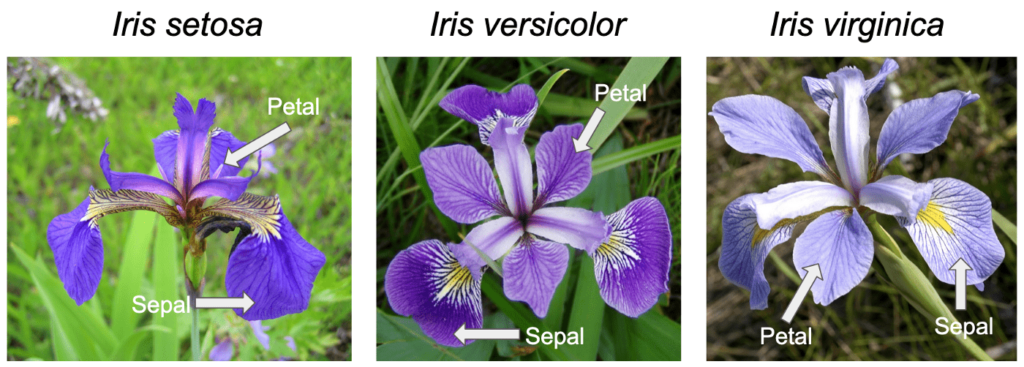
We apply Scikit-learn to the classic Iris dataset, containing measurements of three iris species (setosa, versicolor, and virginica) across four numerical features:

• Sepal Length
  
• Sepal Width
  
• Petal Length
  
• Petal Width

These features capture morphological traits of iris flowers and exhibit strong inter-correlations, making this an ideal dataset to demonstrate how PCA uncovers latent structure and reduces dimensionality.

iris = load_iris()
X = iris.data
y = iris.target
nombres = iris.target_names
feature_names = ['Sepal Length', 'Sepal Width', 'Petal Length', 'Petal Width']

df_iris = pd.DataFrame(X, columns=feature_names)
df_iris['Species'] = [nombres[i] for i in y]
df_iris.describe().round(3)

	Sepal Length	Sepal Width	Petal Length	Petal Width
count	150.000	150.000	150.000	150.000
mean	5.843	3.057	3.758	1.199
std	0.828	0.436	1.765	0.762
min	4.300	2.000	1.000	0.100
25%	5.100	2.800	1.600	0.300
50%	5.800	3.000	4.350	1.300
75%	6.400	3.300	5.100	1.800
max	7.900	4.400	6.900	2.500

Step 1: Standardization

Standardization is mandatory when features operate on differing scales. Without it, features with high raw variance dominate PCA directions regardless of structural importance.

\[ z_{ij} = \frac{x_{ij} - \bar{x}_j}{s_j} \]

Post-standardization: \(\bar{z}_j = 0\) and \(s_{z_j} = 1\) for all features \(j\).

scaler = StandardScaler()
X_std = scaler.fit_transform(X)

df_check = pd.DataFrame({
    'Feature': feature_names,
    'Original Mean': X.mean(axis=0).round(3),
    'Original Std': X.std(axis=0).round(3),
    'Standardized Mean': X_std.mean(axis=0).round(10),
    'Standardized Std': X_std.std(axis=0).round(3)
})
df_check

	Feature	Original Mean	Original Std	Standardized Mean	Standardized Std
0	Sepal Length	5.843	0.825	-0.0	1.0
1	Sepal Width	3.057	0.434	-0.0	1.0
2	Petal Length	3.758	1.759	-0.0	1.0
3	Petal Width	1.199	0.760	-0.0	1.0

Step 2: Covariance Matrix

S = np.cov(X_std.T)

fig = go.Figure(data=go.Heatmap(
    z=S,
    x=feature_names,
    y=feature_names,
    colorscale='RdBu_r',
    zmid=0, zmin=-1, zmax=1,
    text=np.round(S, 3),
    texttemplate='%{text}',
    textfont=dict(size=13),
    hovertemplate='%{y} ↔ %{x}<br>cov = %{z:.3f}<extra></extra>',
    colorbar=dict(title='Covariance')
))
fig.update_layout(
    title="Covariance Matrix — Standardized Data (= Pearson Correlation Matrix)",
    height=420
)
fig.show()

Note

On standardized features, the sample covariance matrix equals the Pearson correlation matrix. PCA on standardized features is equivalent to correlation-based PCA.

Step 3: Eigendecomposition via SVD

pca = PCA()
scores = pca.fit_transform(X_std)

eigenvalues = pca.explained_variance_
pve = pca.explained_variance_ratio_ * 100
pve_acum = np.cumsum(pve)

df_pca = pd.DataFrame({
    'Component': [f'PC{i+1}' for i in range(len(eigenvalues))],
    'Eigenvalue (λ)': eigenvalues.round(4),
    '% Variance': pve.round(2),
    '% Cumulative': pve_acum.round(2)
})
df_pca

	Component	Eigenvalue (λ)	% Variance	% Cumulative
0	PC1	2.9381	72.96	72.96
1	PC2	0.9202	22.85	95.81
2	PC3	0.1477	3.67	99.48
3	PC4	0.0209	0.52	100.00

Step 4: Scree Plot

fig = make_subplots(specs=[[{"secondary_y": True}]])

fig.add_trace(go.Bar(
    x=df_pca['Component'], y=df_pca['% Variance'],
    name='% Variance',
    text=[f"{v:.1f}%" for v in pve],
    textposition='outside'
), secondary_y=False)

fig.add_trace(go.Scatter(
    x=df_pca['Component'], y=pve_acum,
    mode='lines+markers',
    line=dict(width=2.5),
    marker=dict(size=9),
    name='% Cumulative'
), secondary_y=True)

fig.add_hline(y=80, line_dash="dash", line_color="gray",
              annotation_text="80%", secondary_y=True)

fig.update_yaxes(title_text="% Variance per Component", secondary_y=False)
fig.update_yaxes(title_text="% Cumulative Variance", range=[0, 110], secondary_y=True)
fig.update_layout(
    title="Scree Plot — Kaiser Rule: Retain Components with λ > 1",
    height=380
)
fig.show()

Tip

Component Selection Rules (\(k\)):

• Kaiser Rule: retain components with \(\lambda_k > 1\) (applies to standardized data)
• Cumulative Variance: retain components reaching an 80% or 90% cumulative variance threshold
• Scree Plot Elbow: locate the elbow point where variance drop flattens
• Domain Interpretability: confirm selected components represent meaningful domain constructs

Step 5: Biplot

A biplot overlays sample scores and feature loadings in the reduced PC subspace.

loadings = pca.components_
scores_df = pd.DataFrame(scores[:, :2], columns=['PC1', 'PC2'])
scores_df['Species'] = [nombres[i] for i in y]

fig = go.Figure()

# Scores
for especie in nombres:
    mask = scores_df['Species'] == especie
    fig.add_trace(go.Scatter(
        x=scores_df.loc[mask, 'PC1'],
        y=scores_df.loc[mask, 'PC2'],
        mode='markers',
        marker=dict(size=7, opacity=0.7),
        name=especie
    ))

# Scaled loading vectors
escala = 3.0
for i, feat in enumerate(feature_names):
    fig.add_annotation(
        x=loadings[0, i] * escala,
        y=loadings[1, i] * escala,
        ax=0, ay=0,
        arrowhead=3, arrowwidth=2,
        xref='x', yref='y', axref='x', ayref='y',
        showarrow=True
    )
    fig.add_annotation(
        x=loadings[0, i] * escala * 1.15,
        y=loadings[1, i] * escala * 1.15,
        text=f"<b>{feat}</b>",
        showarrow=False,
        font=dict(size=11)
    )

fig.update_xaxes(title_text=f"PC1 ({pve[0]:.1f}%)",
                 zeroline=True, zerolinecolor='lightgray')
fig.update_yaxes(title_text=f"PC2 ({pve[1]:.1f}%)",
                 zeroline=True, zerolinecolor='lightgray',
                 scaleanchor='x')
fig.update_layout(
    title="Biplot: Scores + Loadings — Iris",
    height=480,
    legend=dict(title='Species')
)
fig.show()

Step 6: Detailed Loadings

df_loadings = pd.DataFrame(
    loadings[:2].T,
    index=feature_names,
    columns=['PC1', 'PC2']
).round(4)

fig = make_subplots(
    rows=1, cols=2,
    subplot_titles=[
        "<b>Principal Component 1 (PC1)</b>",
        "<b>Principal Component 2 (PC2)</b>"
    ]
)

# PC1
fig.add_trace(go.Bar(
    x=feature_names,
    y=loadings[0],
    text=[f"{v:.3f}" for v in loadings[0]],
    textposition='outside'
), row=1, col=1)

# PC2
fig.add_trace(go.Bar(
    x=feature_names,
    y=loadings[1],
    text=[f"{v:.3f}" for v in loadings[1]],
    textposition='outside'
), row=1, col=2)

for c in [1, 2]:
    fig.update_yaxes(
        range=[-1.1, 1.1],
        zeroline=True,
        zerolinecolor='lightgray',
        row=1, col=c
    )
    fig.update_xaxes(
        tickangle=-25,
        row=1, col=c
    )

for ann in fig['layout']['annotations']:
    ann['font'] = dict(size=14)

fig.update_layout(
    showlegend=False,
    height=420,
    annotations=list(fig.layout.annotations) + [
        dict(
            x=0.5, y=-0.2,
            xref='paper', yref='paper',
            text="PC1 ≈ overall size | PC2 ≈ sepal structural contrast",
            showarrow=False,
            font=dict(size=12, color='gray'),
            xanchor='center'
        )
    ]
)

fig.show()

---

31 Advanced Example: Noisy Trajectory

Imagine a particle traveling along a 3D helical trajectory measured by noisy multi-sensor arrays. Can PCA recover the underlying trajectory?

31.1 Step 1 — True Trajectory and Sensor Noise

n_points = 500
t = np.linspace(-10, 10, n_points)

# Clean trajectory
x_clean = t
y_clean = np.cos(t)
z_clean = np.sin(t)

# Noisy measurements
sigma = 0.5
y_noise = y_clean + np.random.normal(0, sigma, n_points)
z_noise = z_clean + np.random.normal(0, sigma, n_points)

points = np.column_stack([x_clean, y_noise, z_noise])

fig = go.Figure()

fig.add_trace(go.Scatter3d(
    x=points[:, 0], y=points[:, 1], z=points[:, 2],
    mode='markers',
    marker=dict(size=3, color='steelblue', opacity=0.5),
    name='Noisy Measurements'
))

fig.add_trace(go.Scatter3d(
    x=x_clean, y=y_clean, z=z_clean,
    mode='lines',
    line=dict(color='crimson', width=4),
    name='True Trajectory'
))

fig.update_layout(
    title='Helical Trajectory: True Signal vs. Noisy Sensor Measurements',
    scene=dict(
        xaxis_title='X', yaxis_title='Y', zaxis_title='Z',
        yaxis=dict(range=[-5, 5]),
        xaxis=dict(range=[-11, 11])
    ),
    legend=dict(x=0.01, y=0.99),
    height=520
)
fig.show()

31.2 Step 2 — Three Sensors, Three Perspectives

def proyection(points, plane_point, plane_normal):
    n = plane_normal / np.linalg.norm(plane_normal)
    d = points - plane_point
    dist = d.dot(n)
    return points - np.outer(dist, n)

def plane_axes(plane_normal):
    n = plane_normal / np.linalg.norm(plane_normal)
    arb = np.array([1, 0, 0]) if abs(n[0]) < 0.9 else np.array([0, 1, 0])
    u = np.cross(n, arb)
    u /= np.linalg.norm(u)
    v = np.cross(n, u)
    v /= np.linalg.norm(v)
    return u, v

def sensor_reading(points, plane_point, plane_normal, noise_std=0.5):
    proj_3d = proyection(points, plane_point, plane_normal)
    u, v = plane_axes(plane_normal)
    proj_vectors = proj_3d - plane_point
    s = proj_vectors.dot(u) + np.random.normal(0, noise_std, len(points))
    t = proj_vectors.dot(v) + np.random.normal(0, noise_std, len(points))
    return s, t, proj_3d, u, v

def plane_mesh(plane_point, plane_normal, size=12, res=20):
    u, v = plane_axes(plane_normal)
    lin = np.linspace(-size, size, res)
    uu, vv = np.meshgrid(lin, lin)
    X = plane_point[0] + uu * u[0] + vv * v[0]
    Y = plane_point[1] + uu * u[1] + vv * v[1]
    Z = plane_point[2] + uu * u[2] + vv * v[2]
    return X, Y, Z

sensors = [
    dict(point=np.array([5., -6., 0.]),  normal=np.array([1., -1., 0.]),
         color='royalblue',  name='Sensor A'),
    dict(point=np.array([10., 0., 0.]),  normal=np.array([10., 0., 0.1]),
         color='seagreen',   name='Sensor B'),
    dict(point=np.array([3.,  3., 3.]),  normal=np.array([1.,  1., 1.]),
         color='darkorange', name='Sensor C'),
]

readings = []
for s in sensors:
    sc, tc, proj3d, u, v = sensor_reading(
        points, s['point'], s['normal'], noise_std=0.5
    )
    readings.append({'s': sc, 't': tc, 'proj3d': proj3d,
                     'u': u, 'v': v, **s})

fig = go.Figure()

fig.add_trace(go.Scatter3d(
    x=x_clean, y=y_clean, z=z_clean,
    mode='lines', line=dict(color='crimson', width=4),
    name='True Trajectory'
))

fig.add_trace(go.Scatter3d(
    x=points[:, 0], y=points[:, 1], z=points[:, 2],
    mode='markers', marker=dict(size=2, color='lightgray', opacity=0.4),
    name='Original Measurements'
))

for r in readings:
    px_m, py_m, pz_m = plane_mesh(r['point'], r['normal'], size=10)
    fig.add_trace(go.Surface(
        x=px_m, y=py_m, z=pz_m,
        colorscale=[[0, r['color']], [1, r['color']]],
        opacity=0.15, showscale=False,
        name=f"Plane {r['name']}", showlegend=False
    ))
    fig.add_trace(go.Scatter3d(
        x=r['proj3d'][:, 0], y=r['proj3d'][:, 1], z=r['proj3d'][:, 2],
        mode='markers', marker=dict(size=2.5, color=r['color'], opacity=0.7),
        name=r['name']
    ))

fig.update_layout(
    title='Sensors Projecting Point Cloud Onto Respective Reference Planes',
    scene=dict(xaxis_title='X', yaxis_title='Y', zaxis_title='Z',
               xaxis=dict(range=[-12, 12]),
               yaxis=dict(range=[-8, 8])),
    legend=dict(x=0.01, y=0.99),
    height=560
)
fig.show()

fig = make_subplots(
    rows=1, cols=3,
    subplot_titles=[r['name'] for r in readings],
    shared_yaxes=False
)

for i, r in enumerate(readings, 1):
    fig.add_trace(go.Scatter(
        x=r['s'], y=r['t'],
        mode='markers',
        marker=dict(size=3, color=r['color'], opacity=0.6),
        name=r['name'],
        showlegend=False
    ), row=1, col=i)
    fig.update_xaxes(title_text='u (local plane axis 1)', row=1, col=i,
                     zeroline=True, zerolinecolor='lightgray')
    fig.update_yaxes(title_text='v (local plane axis 2)' if i == 1 else '',
                     row=1, col=i,
                     zeroline=True, zerolinecolor='lightgray')

fig.update_layout(
    title='Raw Sensor Measurements (2D Local Coordinates)',
    height=400
)
fig.show()

31.3 Step 3 — Multi-Sensor Feature Matrix

data_matrix = np.column_stack([
    readings[0]['s'], readings[0]['t'],
    readings[1]['s'], readings[1]['t'],
    readings[2]['s'], readings[2]['t'],
])

col_labels = ['A_u', 'A_v', 'B_u', 'B_v', 'C_u', 'C_v']

corr = np.corrcoef(data_matrix.T)

fig = go.Figure(data=go.Heatmap(
    z=corr,
    x=col_labels, y=col_labels,
    colorscale='RdBu_r',
    zmid=0, zmin=-1, zmax=1,
    text=np.round(corr, 2),
    texttemplate='%{text}',
    textfont=dict(size=11),
    colorbar=dict(title='Correlation')
))

fig.update_layout(
    title='Correlation Across 6 Sensor Variables',
    height=420
)
fig.show()

31.4 Step 4 — PCA Decomposition

pca_full = PCA(n_components=6)
components_full = pca_full.fit_transform(data_matrix)

explained = pca_full.explained_variance_ratio_
cumulative = np.cumsum(explained)

fig = make_subplots(specs=[[{"secondary_y": True}]])

fig.add_trace(go.Bar(
    x=[f'PC{i+1}' for i in range(6)],
    y=explained * 100,
    name='% Variance',
    text=[f'{v*100:.1f}%' for v in explained],
    textposition='outside',
    marker_color='steelblue'
), secondary_y=False)

fig.add_trace(go.Scatter(
    x=[f'PC{i+1}' for i in range(6)],
    y=cumulative * 100,
    mode='lines+markers',
    name='% Cumulative',
    line=dict(color='crimson', width=2.5),
    marker=dict(size=9)
), secondary_y=True)

fig.add_hline(y=90, line_dash='dash', line_color='gray',
              annotation_text='90%', secondary_y=True)

fig.update_yaxes(title_text="% Variance per Component", secondary_y=False)
fig.update_yaxes(title_text="% Cumulative Variance", range=[0, 110],
                 secondary_y=True)
fig.update_layout(
    title='Scree Plot: How Many Components Capture Signal?',
    height=400
)
fig.show()

31.5 Step 5 — 2D Projection

pca_2d = PCA(n_components=2)
proj_2d = pca_2d.fit_transform(data_matrix)

fig = go.Figure()

fig.add_trace(go.Scatter(
    x=proj_2d[:, 0], y=proj_2d[:, 1],
    mode='markers',
    marker=dict(
        size=4, opacity=0.8,
        color=t,
        colorscale='Viridis',
        colorbar=dict(title='t (time)', len=0.6)
    ),
    name='Colored by t'
))

fig.update_xaxes(title_text='Principal Component 1',
                 zeroline=True, zerolinecolor='lightgray')
fig.update_yaxes(title_text='Principal Component 2',
                 zeroline=True, zerolinecolor='lightgray',
                 scaleanchor='x')
fig.update_layout(
    title=f'PC1 vs PC2 — {pca_2d.explained_variance_ratio_.sum()*100:.1f}% Total Variance',
    height=480
)
fig.show()

31.6 Step 6 — 3D Reconstruction

pca_3d = PCA(n_components=3)
proj_3d = pca_3d.fit_transform(data_matrix)

fig = go.Figure()

fig.add_trace(go.Scatter3d(
    x=proj_3d[:, 0], y=proj_3d[:, 1], z=proj_3d[:, 2],
    mode='markers',
    marker=dict(
        size=3, opacity=0.7,
        color=t,
        colorscale='Viridis',
        colorbar=dict(title='t', len=0.5)
    ),
    name='Samples'
))

scale = proj_3d[:, 0].std() / x_clean.std()
fig.add_trace(go.Scatter3d(
    x=x_clean * scale,
    y=y_clean * proj_3d[:, 1].std(),
    z=z_clean * proj_3d[:, 2].std(),
    mode='lines',
    line=dict(color='crimson', width=4),
    name='True Trajectory (scaled)'
))

fig.update_layout(
    title=f'3D Projection — {pca_3d.explained_variance_ratio_.sum()*100:.1f}% Total Variance',
    scene=dict(
        xaxis_title='PC 1',
        yaxis_title='PC 2',
        zaxis_title='PC 3',
        xaxis=dict(range=[-15, 15]),
        yaxis=dict(range=[-7, 7]),
        zaxis=dict(range=[-7, 7])
    ),
    legend=dict(x=0.01, y=0.99),
    height=560
)
fig.show()

NoteCentral Idea

PCA has no prior knowledge of physical trajectories. It isolates maximum variance directions across noisy observations. Because signal variance dominates noise (\(\text{SNR} \gg 1\)), top components capture true signal dynamics.

WarningImportant Limitation

PCA projects onto linear subspaces. Non-linear manifolds require methods like UMAP or t-SNE.