---
title: "Supervised Classifiers: Practical Experiment"
description: "Hands-on Python exercise applying supervised classification algorithms to labeled data, from feature vectors to generalizable prediction models."
pagetitle: "Supervised Classifiers: Practical Experiment"
open-graph:
description: "Hands-on Python exercise applying supervised classification algorithms to labeled data, from feature vectors to generalizable prediction models."
twitter-card:
description: "Hands-on Python exercise applying supervised classification algorithms to labeled data, from feature vectors to generalizable prediction models."
author: "Diego Villalba"
date: today
lang: en
format:
html:
toc: true
toc-depth: 3
toc-title: "Contents"
number-sections: true
code-fold: false
code-tools: true
code-summary: "Show code"
fig-align: center
theme: cosmo
highlight-style: github
smooth-scroll: true
pdf:
toc: true
toc-depth: 3
number-sections: true
documentclass: scrbook
papersize: letter
fontsize: 11pt
geometry: margin=2.5cm
keep-tex: false
execute:
echo: true
warning: false
message: false
cache: false
bibliography: [references_example.bib, ../../../references.bib]
crossref:
fig-title: "Figure"
tbl-title: "Table"
eq-prefix: "Eq."
jupyter: python3
---
```{python}
#| echo: false
#| label: setup-capitulo
import numpy as np
import pandas as pd
import matplotlib.pyplot as plt
import warnings
warnings.filterwarnings("ignore")
import matplotlib
matplotlib.rcParams.update({
"figure.dpi": 100,
"axes.spines.top": False,
"axes.spines.right": False,
"font.size": 11,
})
SEED = 42
np.random.seed(SEED)
```
# Introduction
Supervised classification is one of the central tasks of machine learning. Given a set of labeled observations $\{(\mathbf{x}_i, y_i)\}_{i=1}^{n}$, where $\mathbf{x}_i \in \mathbb{R}^d$ is the feature vector and $y_i \in \{0, 1, \ldots, K-1\}$ is the target class, the classification problem consists of learning a mapping $f: \mathbb{R}^d \to \mathcal{Y}$ that generalizes accurately to unseen future observations.
This chapter does not focus on deriving theoretical algorithms from scratch, but rather on demonstrating how to design, execute, and evaluate a practical end-to-end classification experiment. The emphasis is on real-world workflow challenges: proper data preparation, avoiding data leakage, establishing fair benchmark comparisons, and interpreting metrics within specific problem domains.
---
# Dataset: Breast Cancer Wisconsin
The Breast Cancer Wisconsin dataset [@wolberg1995breast] contains 569 tissue biopsy samples, each described by 30 numerical features computed from digitized cell images. The target label indicates whether a tumor is malignant (0) or benign (1). This dataset exhibits key pedagogical properties:
- Available directly within scikit-learn without external downloads;
- Fully numerical feature space, simplifying preprocessing pipelines;
- Clear domain motivation with asymmetric error consequences;
- Moderate class imbalance (37% malignant, 63% benign), ideal for metric comparison discussions.
```{python}
#| label: carga-capitulo
#| code-fold: false
from sklearn.datasets import load_breast_cancer

data = load_breast_cancer()
X = pd.DataFrame(data.data, columns=data.feature_names)
y = pd.Series(data.target, name="target")

print(f"Dataset shape: {X.shape}")
print("Class distribution:")
print(y.value_counts().rename({0: "Malignant (0)", 1: "Benign (1)"}))
```
In scikit-learn, `target=1` corresponds to benign and `target=0` to malignant. When evaluating precision and recall, specifying target class assignment is essential, as values vary significantly depending on class focus.
---
# General Workflow for a Classification Experiment
A well-structured classification experiment follows these systematic steps:
1. **Problem Definition:** Understand the domain goal and target variable.
2. **Exploratory Analysis & Preprocessing:** Inspect feature distributions and clean data.
3. **Data Partitioning:** Split data into train and test sets strictly prior to preprocessing.
4. **Model Selection:** Establish baseline classifiers and initial hyperparameter configurations.
5. **Model Training:** Fit estimators using training data exclusively.
6. **Performance Evaluation:** Measure model performance using domain-aligned metrics.
7. **Model Comparison:** Evaluate all candidate estimators on identical test splits.
8. **Threshold Optimization:** Tune decision thresholds based on error costs.
9. **Result Interpretation:** Inspect decision boundaries, feature importances, and limitations.
10. **Documentation:** Record all random seeds, library versions, and pipeline parameters for reproducibility.
---
# Data Preparation
## Train/Test Partitioning
The gold standard in experimental design requires withholding the test set completely during model design, feature scaling, and hyperparameter tuning. Using test set information during design introduces **data leakage**, leading to overly optimistic performance estimates that fail in production.
```{python}
#| label: split-capitulo
#| code-fold: false
from sklearn.model_selection import train_test_split

X_train, X_test, y_train, y_test = train_test_split(
    X, y,
    test_size=0.2,
    random_state=SEED,
    stratify=y
)

print(f"Training set: {X_train.shape[0]} samples")
print(f"Test set:     {X_test.shape[0]} samples")
```
Setting `stratify=y` ensures class proportions remain consistent across training and test splits, which is vital under class imbalance.
## Leak-Free Preprocessing via Pipelines
Applying transformations such as feature scaling must be encapsulated inside a scikit-learn `Pipeline` [@pedregosa2011]. A pipeline guarantees that transformer fitting (e.g., `StandardScaler`) occurs strictly on training data, while applying the fitted transformation automatically to test instances.
```{python}
#| label: pipeline-capitulo
from sklearn.pipeline import Pipeline
from sklearn.preprocessing import StandardScaler
from sklearn.linear_model import LogisticRegression

pipe = Pipeline([
    ("scaler", StandardScaler()),
    ("clf",    LogisticRegression(max_iter=1000, random_state=SEED))
])

pipe.fit(X_train, y_train)
print(f"Test Accuracy: {pipe.score(X_test, y_test):.4f}")
```
A common data leakage flaw occurs when transformers fit on the full dataset prior to splitting:
```python
# ✗ INCORRECT: StandardScaler fit on full X (includes test data)
scaler = StandardScaler()
X_scaled = scaler.fit_transform(X)
X_train_s, X_test_s = train_test_split(X_scaled, ...)
```
## Cross-Validation
On small datasets, single train/test split evaluations can suffer from sample variance. $k$-fold cross-validation [@kohavi1995] partitions training data into $k$ disjoint folds, training $k$ models on $k-1$ folds and evaluating on the remaining fold, reporting average cross-validation scores.
```{python}
#| label: cv-capitulo
from sklearn.model_selection import cross_val_score
from sklearn.ensemble import RandomForestClassifier

pipe_rf = Pipeline([
    ("clf", RandomForestClassifier(n_estimators=100, random_state=SEED))
])

scores = cross_val_score(pipe_rf, X_train, y_train, cv=5, scoring="f1")
print(f"F1 per fold: {np.round(scores, 4)}")
print(f"Mean F1:    {scores.mean():.4f}  ±  {scores.std():.4f}")
```
Cross-validation serves for hyperparameter tuning and model selection; the held-out test set remains the final benchmark of generalization.
---
# Classifiers: Intuition, Inductive Biases, and Hyperparameters
## Logistic Regression (Baseline)
Logistic regression models positive class probability via the sigmoid activation function applied to a linear combination of input features:
$$P(y=1 \mid \mathbf{x}) = \sigma(\mathbf{w}^\top \mathbf{x} + b) = \frac{1}{1 + e^{-(\mathbf{w}^\top \mathbf{x} + b)}}$$
It serves as a standard interpretable linear baseline. Coefficients indicate individual feature contributions. **Requires feature scaling** for gradient convergence and coefficient comparability.
Key hyperparameters:
- `C`: Inverse regularization strength (smaller values $\implies$ stronger regularization)
- `penalty`: Norm penalty type (`l1`, `l2`, `elasticnet`)
- `max_iter`: Maximum optimizer iterations
## Decision Trees: CART and ID3
### CART [@breiman1984]
CART (*Classification and Regression Trees*) builds binary trees via recursive feature space partitioning. At each node, it selects the split threshold minimizing Gini impurity:
$$G = 1 - \sum_{k=0}^{K-1} p_k^2$$
where $p_k$ is the proportion of class $k$ samples at the node.
### ID3 [@quinlan1986id3]
ID3 (*Iterative Dichotomiser 3*) uses Information Gain based on entropy:
$$\text{Gain}(S, A) = H(S) - \sum_{v \in \text{Values}(A)} \frac{|S_v|}{|S|} H(S_v)$$
where $H(S) = -\sum_k p_k \log_2 p_k$. In scikit-learn, ID3 is approximated setting `criterion="entropy"` in `DecisionTreeClassifier`.
Key tree hyperparameters:
- `max_depth`: Maximum depth tree expansion
- `min_samples_split`: Minimum sample count required to split a node
- `min_samples_leaf`: Minimum sample count required at a leaf node
```{python}
#| label: cart-hiperparametros
from sklearn.tree import DecisionTreeClassifier
from sklearn.metrics import f1_score

for criterion in ["gini", "entropy"]:
    for depth in [3, 5, None]:
        pipe = Pipeline([
            ("clf", DecisionTreeClassifier(
                criterion=criterion, max_depth=depth, random_state=SEED
            ))
        ])
        pipe.fit(X_train, y_train)
        f1 = f1_score(y_test, pipe.predict(X_test))
        print(f"criterion={criterion:7s} | max_depth={str(depth):5s} | F1={f1:.4f}")
```
## Random Forest [@breiman2001]
Random Forest is a parallel ensemble of decision trees trained via bootstrap aggregating (bagging). Each tree trains on a random bootstrap sample with replacement, while node splits evaluate a random subset of features (`max_features`), decorrelating individual trees and reducing variance.
Key hyperparameters:
- `n_estimators`: Number of trees in ensemble
- `max_features`: Random feature subset size per split (`sqrt`, `log2`)
- `max_depth`: Maximum tree depth
- `min_samples_leaf`: Minimum leaf sample count
```{python}
#| label: rf-capitulo
from sklearn.ensemble import RandomForestClassifier
from sklearn.metrics import roc_auc_score

pipe_rf = Pipeline([
    ("clf", RandomForestClassifier(
        n_estimators=100, max_depth=None, random_state=SEED
    ))
])
pipe_rf.fit(X_train, y_train)
f1 = f1_score(y_test, pipe_rf.predict(X_test))
auc = roc_auc_score(y_test, pipe_rf.predict_proba(X_test)[:,1])
print(f"Random Forest — F1={f1:.4f}  AUC={auc:.4f}")
```
## Gradient Boosting [@friedman2001gradient]
Gradient Boosting builds tree ensembles **sequentially**. Each new weak learner is trained to predict residual errors of the accumulated ensemble, minimizing loss via functional gradient descent.
XGBoost [@chen2016xgboost] provides an optimized gradient boosting implementation featuring explicit L1/L2 tree regularization, fast approximate split finding, and native missing value handling.
Key hyperparameters:
- `n_estimators`: Sequential tree count
- `learning_rate`: Step size shrinkage factor (typically 0.01–0.3)
- `max_depth`: Tree depth per weak learner (typically 3–6)
- `subsample`: Row subsample ratio
```{python}
#| label: gb-capitulo
from sklearn.ensemble import GradientBoostingClassifier

pipe_gb = Pipeline([
    ("clf", GradientBoostingClassifier(
        n_estimators=100, learning_rate=0.1,
        max_depth=3, random_state=SEED
    ))
])
pipe_gb.fit(X_train, y_train)
f1 = f1_score(y_test, pipe_gb.predict(X_test))
auc = roc_auc_score(y_test, pipe_gb.predict_proba(X_test)[:,1])
print(f"Gradient Boosting — F1={f1:.4f}  AUC={auc:.4f}")
```
## Multilayer Perceptron (MLP)
A Multilayer Perceptron (MLP) neural network models non-linear functions via composition of affine transformations and non-linear activation functions [@bishop2006; @goodfellow2016deep]:
$$\mathbf{h}^{(l)} = \sigma\!\left(\mathbf{W}^{(l)} \mathbf{h}^{(l-1)} + \mathbf{b}^{(l)}\right)$$
where $\sigma$ is an activation function (ReLU, tanh), $\mathbf{W}^{(l)}$ represents weight matrices, and $\mathbf{h}^{(0)} = \mathbf{x}$. Weights are optimized using backpropagation.
MLPs require feature scaling: unscaled inputs with disparate variances lead to unstable gradients and optimizer failure.
```{python}
#| label: mlp-capitulo
from sklearn.neural_network import MLPClassifier

# With feature scaling (correct)
pipe_mlp = Pipeline([
    ("scaler", StandardScaler()),
    ("clf", MLPClassifier(
        hidden_layer_sizes=(64, 32),
        max_iter=300, random_state=SEED
    ))
])
pipe_mlp.fit(X_train, y_train)
f1 = f1_score(y_test, pipe_mlp.predict(X_test))
auc = roc_auc_score(y_test, pipe_mlp.predict_proba(X_test)[:,1])
print(f"MLP (with scaling)    — F1={f1:.4f}  AUC={auc:.4f}")

# Without feature scaling (demonstration of failure)
pipe_mlp_raw = Pipeline([
    ("clf", MLPClassifier(
        hidden_layer_sizes=(64, 32),
        max_iter=300, random_state=SEED
    ))
])
pipe_mlp_raw.fit(X_train, y_train)
f1_raw = f1_score(y_test, pipe_mlp_raw.predict(X_test))
auc_raw = roc_auc_score(y_test, pipe_mlp_raw.predict_proba(X_test)[:,1])
print(f"MLP (without scaling) — F1={f1_raw:.4f}  AUC={auc_raw:.4f}")
```
---
# Review of Evaluation Metrics
Derived from the confusion matrix:
$$\text{Accuracy} = \frac{TP + TN}{TP + TN + FP + FN}$$
$$\text{Precision} = \frac{TP}{TP + FP}$$
$$\text{Recall (Sensitivity)} = \frac{TP}{TP + FN}$$
$$F_1 = \frac{2 \cdot \text{Precision} \cdot \text{Recall}}{\text{Precision} + \text{Recall}}$$
[@powers2011; @pedregosa2011]
## ROC Curve and AUC
The ROC curve [@fawcett2006] plots True Positive Rate vs. False Positive Rate across all decision thresholds. Area Under the Curve (AUC) summarizes global discriminative capacity into a single scalar ($AUC=1.0$ is perfect; $AUC=0.5$ is random guessing).
## Precision–Recall Curve and Average Precision
The Precision–Recall curve [@saito2015] plots Precision vs. Recall across all thresholds. It is vastly superior to ROC when evaluating rare positive classes, as ROC curves can appear deceptively optimistic under high True Negative counts. Average Precision (AP) measures the area under the PR curve.
---
# Decision Threshold Optimization
## Motivation
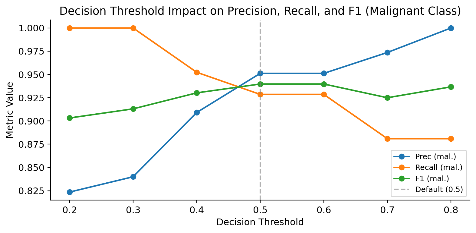
By default, `predict()` maps continuous probabilities to binary predictions using cut-off $\theta = 0.5$. However, default thresholds are rarely optimal under asymmetric error costs. In oncology screening, missing a malignant tumor (False Negative) carries far worse consequences than ordering a follow-up biopsy (False Positive).
## Evaluating Threshold Cut-offs
```{python}
#| label: thresholds-capitulo
from sklearn.metrics import precision_score, recall_score, f1_score

probs_mal = pipe_rf.predict_proba(X_test)[:, 0]
thresholds = [0.20, 0.30, 0.40, 0.50, 0.60, 0.70, 0.80]

filas = []
for th in thresholds:
    y_pred = np.where(probs_mal >= th, 0, 1)
    filas.append({
        "Threshold":     th,
        "Prec (mal.)":   precision_score(y_test, y_pred, pos_label=0, zero_division=0),
        "Recall (mal.)": recall_score(y_test, y_pred, pos_label=0, zero_division=0),
        "F1 (mal.)":     f1_score(y_test, y_pred, pos_label=0, zero_division=0),
        "FN":            ((y_pred == 1) & (y_test.values == 0)).sum(),
        "FP":            ((y_pred == 0) & (y_test.values == 1)).sum(),
    })

df_th = pd.DataFrame(filas).set_index("Threshold")
print(df_th.round(4).to_string())
```
```{python}
#| label: viz-thresholds-capitulo
fig, ax = plt.subplots(figsize=(8, 4))
df_th[["Prec (mal.)", "Recall (mal.)", "F1 (mal.)"]].plot(ax=ax, marker="o", linewidth=1.8)
ax.axvline(0.5, color="gray", linestyle="--", alpha=0.6, label="Default (0.5)")
ax.set_xlabel("Decision Threshold")
ax.set_ylabel("Metric Value")
ax.set_title("Decision Threshold Impact on Precision, Recall, and F1 (Malignant Class)")
ax.legend(fontsize=9)
plt.tight_layout()
plt.show()
```
---
# Model Comparison
Fair comparison requires evaluating all models on the **exact same test set**, applying **consistent preprocessing**, and measuring **identical domain metrics**.
```{python}
#| label: comparacion-capitulo
from sklearn.metrics import accuracy_score

modelos_todos = {
    "Logistic Regression": Pipeline([
        ("scaler", StandardScaler()),
        ("clf", LogisticRegression(max_iter=1000, random_state=SEED))
    ]),
    "CART (Gini)": Pipeline([
        ("clf", DecisionTreeClassifier(criterion="gini", max_depth=5, random_state=SEED))
    ]),
    "ID3-proxy (Entropy)": Pipeline([
        ("clf", DecisionTreeClassifier(criterion="entropy", max_depth=5, random_state=SEED))
    ]),
    "Random Forest": Pipeline([
        ("clf", RandomForestClassifier(n_estimators=100, random_state=SEED))
    ]),
    "Gradient Boosting": Pipeline([
        ("clf", GradientBoostingClassifier(
            n_estimators=100, learning_rate=0.1, max_depth=3, random_state=SEED
        ))
    ]),
    "MLP Neural Net": Pipeline([
        ("scaler", StandardScaler()),
        ("clf", MLPClassifier(hidden_layer_sizes=(64, 32), max_iter=300, random_state=SEED))
    ]),
}

filas_comp = []
for nombre, pipe in modelos_todos.items():
    pipe.fit(X_train, y_train)
    y_pred = pipe.predict(X_test)
    y_prob = pipe.predict_proba(X_test)[:, 1]
    filas_comp.append({
        "Model":     nombre,
        "Accuracy":  accuracy_score(y_test, y_pred),
        "F1":        f1_score(y_test, y_pred),
        "ROC-AUC":   roc_auc_score(y_test, y_prob),
        "Recall":    recall_score(y_test, y_pred),
        "Precision": precision_score(y_test, y_pred),
    })

df_comp = pd.DataFrame(filas_comp).set_index("Model")
print(df_comp.sort_values("ROC-AUC", ascending=False).round(4).to_string())
```
---
# Best Practices for Supervised Experiments
1. **Encapsulate Preprocessing in Pipelines:** Prevent data leakage by nesting scalers and classifiers.
2. **Fix Random Seeds:** Pass `random_state` across splits and stochastic estimators.
3. **Stratify Splits:** Preserve class ratios using `stratify=y`.
4. **Evaluate on Identical Test Splits:** Ensure fair head-to-head model comparison.
5. **Report Multiple Metrics:** Complement accuracy with F1, ROC-AUC, and PR-AUC.
6. **Tune Hyperparameters via Validation Sets:** Never use the test set for hyperparameter optimization.
7. **Inspect Confusion Matrices:** Contextualize aggregate metrics with raw error counts.
---
# Common Pitfalls in Classification Experiments
- **Evaluating on Training Data:** Produces deceptive performance figures due to overfitting.
- **Scaling Prior to Splitting:** Causes data leakage across train/test boundaries.
- **Relying Solely on Accuracy:** Misleading under class imbalance.
- **Failing to Scale Inputs for Neural Networks / Logistic Regression:** Leads to optimizer failure and degraded performance.
- **Re-using Test Sets for Design Iteration:** Overfits models to test sets.
---
# Conclusions
Designing a valid classification experiment requires far more than calling `.fit()`. Data partitioning choices, leak-free preprocessing, metric selection, model benchmarking, and threshold optimization directly govern experimental validity.
The models evaluated — Logistic Regression, CART, ID3, Random Forest, Gradient Boosting, and MLP — represent distinct inductive biases and trade-offs among interpretability, flexibility, and performance. No single model is universally superior; estimator selection must align with data volume, feature types, and operational requirements.
## References {.unnumbered}
::: {#refs}
:::