39  Classification and Decision Trees

1 Introduction

Classification is one of the fundamental tasks in supervised learning. Its goal is to learn a decision rule from previously observed examples capable of assigning a categorical label to new observations. Unlike numerical prediction (regression), where the output belongs to a continuous or ordered discrete space, in classification the output belongs to a finite set of discrete classes: for example, spam or non-spam, approve or reject, positive, negative, or neutral (Hastie et al. 2009; James et al. 2021).

In general terms, a classification problem starts with a training dataset composed of pairs

\[ \mathcal{D} = \{(\mathbf{x}_i, y_i)\}_{i=1}^{n}, \]

where \(\mathbf{x}_i \in \mathcal{X}\) represents the predictor variables or available observations, while \(y_i \in \mathcal{Y}\) represents the target class. The objective is to construct a function

\[ \hat{f}: \mathcal{X} \to \mathcal{Y} \]

that generalizes well to unseen data.

This chapter explores decision trees as interpretable classification models. The exposition focuses on the general logic of tree induction, Hunt’s algorithm, the ID3 algorithm, entropy, information gain, and the extraction of classification rules.

2 Classification as a Supervised Problem

In a classification problem, historical examples are available where the true class is known. The model leverages these examples to learn patterns connecting explanatory variables to target labels.

Typical examples include:

• Classifying an email as spam or non-spam;
• Deciding whether a credit application should be approved or rejected;
• Identifying whether a patient presents hypertension;
• Categorizing a review as positive, negative, or neutral;
• Predicting whether a customer will purchase a laptop.

The distinction between classification and regression depends on the type of target variable. If the output is categorical, it is a classification problem. If the output is numerical, it is a regression problem.

Task	Output Type	Example
Classification	Categorical	Pass / Fail
Regression	Numerical	Tomorrow’s Temperature

Definition. A supervised classification problem consists of estimating a function \(\hat{f}\) that maps each observation \(\mathbf{x}\) to a class \(y\) within a finite set of labels \(\mathcal{Y}\): \[ \hat{f}: \mathcal{X} \to \mathcal{Y}, \qquad |\mathcal{Y}| < \infty. \tag{1}\]

3 Training, Testing, and Generalization

Classification workflows are typically divided into two main phases: training and testing. During training, the algorithm adjusts its internal rules using labeled data. During testing, the model is evaluated on unseen data to estimate its generalization capability.

This separation is essential because a model can memorize training data without learning useful underlying patterns. This phenomenon is known as overfitting. In decision trees, overfitting occurs when a tree grows too deep, creating highly specific partitions for individual training cases (Breiman et al. 1984; Quinlan 1986).

Definition. Given a training set \(\mathcal{D}_{\text{train}}\) and a test set \(\mathcal{D}_{\text{test}}\), the generalization capability of a classifier is evaluated by estimating its performance on examples not used during model fitting: \[ \mathcal{D} = \mathcal{D}_{\text{train}} \cup \mathcal{D}_{\text{test}}, \qquad \mathcal{D}_{\text{train}} \cap \mathcal{D}_{\text{test}} = \varnothing. \tag{2}\]

4 Data Preparation Before Classifier Building

Before training a classifier, data preparation is required. Model quality depends directly on feature quality. Three common tasks are data cleaning, transformation, and dimensionality reduction.

Data cleaning involves correcting invalid or inconsistent entries (such as negative ages or misspelled categories) and deciding how to handle missing values. Data transformation includes encoding categorical variables, scaling numerical features, and parsing dates into usable features. Dimensionality reduction removes redundant, irrelevant, or noisy features.

For decision trees, feature scaling is less critical than in linear models or neural networks, as trees are invariant to monotonic feature transformations. However, category quality, missing value strategies, and handling of continuous features remain important considerations (James et al. 2021; Géron 2022).

import pandas as pd

clientes = pd.DataFrame({
    "income": ["high", "low", "medium", "low", "medium"],
    "credit_history": ["good", "bad", "good", "fair", "bad"],
    "debt": ["low", "high", "low", "high", "medium"],
    "stable_employment": ["yes", "no", "yes", "no", "yes"],
    "decision": ["approve", "reject", "approve", "reject", "reject"]
})

clientes

	income	credit_history	debt	stable_employment	decision
0	high	good	low	yes	approve
1	low	bad	high	no	reject
2	medium	good	low	yes	approve
3	low	fair	high	no	reject
4	medium	bad	medium	yes	reject

The example above represents a binary classification task: deciding whether to approve or reject a credit application. Predictor variables are categorical, and the target label is decision.

5 Decision Trees

A decision tree is a predictive model that organizes sequential decisions in a hierarchical structure. Each internal node represents a test on an attribute, each branch represents a test outcome, and each leaf node assigns a class. Predicting a new observation involves traversing the tree from the root to a leaf.

Decision trees are particularly valued for their interpretability. Unlike opaque models, a tree can be translated directly into human-readable IF-THEN rules (Breiman et al. 1984; Quinlan 1993).

Definition. A classification decision tree is a hierarchical structure composed of internal nodes, branches, and leaves. Each internal node applies a test \(h_j(\mathbf{x})\), each branch corresponds to a test outcome, and each leaf assigns a class \(c \in \mathcal{Y}\): \[ T(\mathbf{x}) = c, \qquad c \in \mathcal{Y}. \tag{3}\]

Core elements of a tree include:

Element	Description
Root Node	The topmost node containing all training examples before splitting.
Internal Node	A node where an attribute test is evaluated to split the dataset.
Branch	A outcome path originating from a node test.
Leaf Node	A terminal node assigning a final class label.

6 Data Partitioning in Decision Trees

Tree induction relies on recursively partitioning data. At each node, an attribute is chosen to split the dataset into subsets.

For categorical attributes, the tree may create one branch per category. For instance, if Outlook takes values Sunny, Overcast, and Rain, three branches are formed. In binary trees, categories are evaluated via boolean tests like “Is color red?”.

For continuous attributes, a split threshold must be selected. For example, Income might be split into Income <= 25000 and Income > 25000. Although ID3 was designed primarily for categorical features, extensions such as C4.5 handle continuous variables smoothly (Quinlan 1986, 1993).

7 Hunt’s Algorithm

Hunt’s algorithm outlines a general recursive framework for building decision trees. The core logic is simple: if all examples reaching a node belong to the same class, the node becomes a leaf. Otherwise, an attribute test is chosen to partition the data, and the procedure recurses on each subset.

Let \(D_t\) be the set of training records reaching node \(t\). The algorithm proceeds as follows:

1. If all records in \(D_t\) belong to class \(y\), create a leaf node with label \(y\).
2. If \(D_t\) is empty, create a leaf node labeled with a default class (typically the majority class of the parent node).
3. If records belong to multiple classes, select an attribute test to split \(D_t\).
4. Partition \(D_t\) into subsets based on test outcomes.
5. Recursively apply the algorithm to each subset.

This approach is top-down (moving from root to leaves) and follows a divide-and-conquer strategy.

Definition. Let \(D_t\) be the set of examples reaching node \(t\). A node is pure if all examples in \(D_t\) belong to the exact same class: \[ \exists c \in \mathcal{Y} \; \text{such that} \; y_i = c \quad \forall (\mathbf{x}_i,y_i) \in D_t. \tag{4}\]

8 Stopping Criteria

Tree partitioning cannot continue indefinitely. Common stopping criteria include:

• All examples at the node belong to a single class;
• No remaining attributes are available for splitting;
• The number of examples at the node falls below a minimum threshold;
• Maximum tree depth has been reached;
• Information gain from further splitting falls below a minimum threshold.

In classic ID3, if no attributes remain and examples belong to multiple classes, the node is assigned the majority class label.

9 ID3: Feature Selection via Information Gain

ID3 (Iterative Dichotomiser 3) is a classic decision tree algorithm proposed by Quinlan. It uses information gain at each node to select the attribute that best separates the target classes (Quinlan 1986).

The intuition is that a good splitting attribute produces subsets that are purer (more homogeneous) than the original set. To quantify impurity, ID3 uses entropy from information theory (Shannon 1948).

The workflow is:

1. Start with all training records at the root node.
2. Calculate current dataset entropy.
3. Evaluate all available candidate attributes.
4. Compute weighted average entropy after splitting for each attribute.
5. Select the attribute yielding highest Information Gain.
6. Recurse on child branches.

10 Entropy as an Impurity Measure

Entropy measures the degree of randomness or impurity in a dataset. If all examples belong to a single class, entropy is 0. If classes are evenly split, entropy reaches its maximum value.

Definition. Let \(S\) be a dataset with \(c\) target classes, and let \(p_i\) be the proportion of examples belonging to class \(i\). The entropy of \(S\) is defined as: \[ H(S) = -\sum_{i=1}^{c} p_i \log_2(p_i). \tag{5}\]

By convention, \(0\log_2(0)=0\), since \(\lim_{p \to 0^+} p\log_2(p) = 0\).

For example, if \(S\) contains 15 records with 9 Yes and 6 No labels:

\[ p(\text{Yes}) = \frac{9}{15}, \qquad p(\text{No}) = \frac{6}{15}. \]

Thus,

\[ H(S) = -\frac{9}{15}\log_2\left(\frac{9}{15}\right) -\frac{6}{15}\log_2\left(\frac{6}{15}\right) \approx 0.971. \]

import numpy as np

def entropy(labels):
    values, counts = np.unique(labels, return_counts=True)
    probs = counts / counts.sum()
    return -np.sum(probs * np.log2(probs))

labels = ["Yes"] * 9 + ["No"] * 6
entropy(labels)

np.float64(0.9709505944546686)

11 Information Gain

Information Gain measures the reduction in entropy achieved by partitioning a dataset on a given attribute. A split producing pure child nodes yields high information gain.

Definition. Let \(S\) be a dataset and \(A\) an attribute taking values \(v \in \operatorname{Values}(A)\). If \(S_v\) denotes the subset of examples where attribute \(A\) takes value \(v\), Information Gain is defined as: \[ \operatorname{Gain}(S,A) = H(S) - \sum_{v\in \operatorname{Values}(A)} \frac{|S_v|}{|S|} H(S_v). \tag{6}\]

The first term, \(H(S)\), represents initial dataset impurity. The second term represents expected entropy after splitting, weighted by subset sizes. Information Gain reflects the impurity reduction obtained by splitting on \(A\).

12 Example: Building a Tree for Baseball Game Prediction

Consider a dataset predicting whether a baseball game will be played (Play). Predictor features are Outlook, Temperature, Humidity, and Wind.

import pandas as pd

df = pd.DataFrame({
    "Outlook": [
        "Sunny", "Sunny", "Overcast", "Rain", "Rain",
        "Rain", "Overcast", "Sunny", "Sunny", "Rain",
        "Sunny", "Overcast", "Overcast", "Rain", "Sunny"
    ],
    "Temperature": [
        "Hot", "Hot", "Hot", "Mild", "Cool",
        "Cool", "Cool", "Mild", "Cool", "Mild",
        "Mild", "Mild", "Hot", "Mild", "Cool"
    ],
    "Humidity": [
        "High", "High", "High", "High", "Normal",
        "Normal", "Normal", "High", "Normal", "Normal",
        "Normal", "High", "Normal", "High", "High"
    ],
    "Wind": [
        "Weak", "Strong", "Weak", "Weak", "Weak",
        "Strong", "Strong", "Weak", "Weak", "Weak",
        "Weak", "Strong", "Weak", "Strong", "Weak"
    ],
    "Play": [
        "No", "No", "Yes", "Yes", "Yes",
        "No", "Yes", "No", "Yes", "Yes",
        "Yes", "Yes", "Yes", "No", "No"
    ]
})

df

	Outlook	Temperature	Humidity	Wind	Play
0	Sunny	Hot	High	Weak	No
1	Sunny	Hot	High	Strong	No
2	Overcast	Hot	High	Weak	Yes
3	Rain	Mild	High	Weak	Yes
4	Rain	Cool	Normal	Weak	Yes
5	Rain	Cool	Normal	Strong	No
6	Overcast	Cool	Normal	Strong	Yes
7	Sunny	Mild	High	Weak	No
8	Sunny	Cool	Normal	Weak	Yes
9	Rain	Mild	Normal	Weak	Yes
10	Sunny	Mild	Normal	Weak	Yes
11	Overcast	Mild	High	Strong	Yes
12	Overcast	Hot	Normal	Weak	Yes
13	Rain	Mild	High	Strong	No
14	Sunny	Cool	High	Weak	No

First, compute initial dataset entropy:

H_total = entropy(df["Play"])
H_total

np.float64(0.9709505944546686)

With 9 Yes and 6 No instances, initial entropy is approximately \(0.971\).

Next, evaluate Information Gain for each attribute:

def information_gain(data, attribute, target):
    total_entropy = entropy(data[target])
    weighted_entropy = 0.0
    for value, subset in data.groupby(attribute):
        weight = len(subset) / len(data)
        weighted_entropy += weight * entropy(subset[target])
    return total_entropy - weighted_entropy

attributes = ["Outlook", "Temperature", "Humidity", "Wind"]

gains = {
    attr: information_gain(df, attr, "Play")
    for attr in attributes
}

pd.Series(gains).sort_values(ascending=False)

Outlook        0.279982
Humidity       0.185805
Wind           0.059773
Temperature    0.013315
dtype: float64

Gain values are approximately:

Attribute	Information Gain
Outlook	0.280
Humidity	0.186
Wind	0.145
Temperature	0.013

Outlook yields the highest gain and is selected as the root node.

13 Branch Construction Following Root Selection

Splitting on Outlook creates three child branches:

• Outlook = Overcast;
• Outlook = Sunny;
• Outlook = Rain.

For Outlook = Overcast, all 4 examples belong to class Yes (\(H = 0\)), forming a pure leaf node.

df[df["Outlook"] == "Overcast"]

	Outlook	Temperature	Humidity	Wind	Play
2	Overcast	Hot	High	Weak	Yes
6	Overcast	Cool	Normal	Strong	Yes
11	Overcast	Mild	High	Strong	Yes
12	Overcast	Hot	Normal	Weak	Yes

For Outlook = Sunny, class mixture remains (2 Yes, 4 No), requiring further evaluation on remaining features: Temperature, Humidity, Wind.

sunny = df[df["Outlook"] == "Sunny"]
remaining = ["Temperature", "Humidity", "Wind"]

pd.Series({
    attr: information_gain(sunny, attr, "Play")
    for attr in remaining
}).sort_values(ascending=False)

Humidity       0.918296
Temperature    0.251629
Wind           0.109170
dtype: float64

Humidity yields the highest gain (0.918). Splitting on Humidity:

• Outlook = Sunny and Humidity = High \(\implies\) Play = No;
• Outlook = Sunny and Humidity = Normal \(\implies\) Play = Yes.

For Outlook = Rain, evaluating remaining features identifies Wind as the top splitter (gain = 0.971).

rain = df[df["Outlook"] == "Rain"]

pd.Series({
    attr: information_gain(rain, attr, "Play")
    for attr in remaining
}).sort_values(ascending=False)

Wind           0.970951
Temperature    0.019973
Humidity       0.019973
dtype: float64

Splitting on Wind:

• Outlook = Rain and Wind = Weak \(\implies\) Play = Yes;
• Outlook = Rain and Wind = Strong \(\implies\) Play = No.

14 Final Tree Structure

The final decision tree is summarized as:

flowchart TD
    A[Outlook]
    A -->|Overcast| B[Yes]
    A -->|Sunny| C[Humidity]
    A -->|Rain| D[Wind]
    C -->|High| E[No]
    C -->|Normal| F[Yes]
    D -->|Weak| G[Yes]
    D -->|Strong| H[No]

flowchart TD
    A[Outlook]
    A -->|Overcast| B[Yes]
    A -->|Sunny| C[Humidity]
    A -->|Rain| D[Wind]
    C -->|High| E[No]
    C -->|Normal| F[Yes]
    D -->|Weak| G[Yes]
    D -->|Strong| H[No]

Notice that not all features are required across all branches. In the Overcast branch, Temperature, Humidity, and Wind are unused because class determination is complete.

ID3 Algorithm — Step-by-Step Construction
Dataset: Play Baseball?  ·  n = 15 examples  ·  4 attributes

15 Extracting Classification Rules

A primary benefit of decision trees is their direct conversion into classification rules. Each root-to-leaf path produces a single IF-THEN rule.

From the tree above, we extract:

1. IF Outlook = Sunny AND Humidity = High, THEN Play = No.
2. IF Outlook = Sunny AND Humidity = Normal, THEN Play = Yes.
3. IF Outlook = Overcast, THEN Play = Yes.
4. IF Outlook = Rain AND Wind = Weak, THEN Play = Yes.
5. IF Outlook = Rain AND Wind = Strong, THEN Play = No.

Definition. A classification rule extracted from a decision tree is a logical implication comprising conditions along a root-to-leaf path: \[ \text{IF } (A_1=v_1) \land (A_2=v_2) \land \cdots \land (A_k=v_k) \text{ THEN } y=c. \tag{7}\]

These rules are intuitive and easy to communicate to non-technical domain experts. Consequently, decision trees are widely applied in medical diagnostics, credit scoring, predictive maintenance, and customer churn analysis (Breiman et al. 1984; James et al. 2021).

16 Implementation with scikit-learn

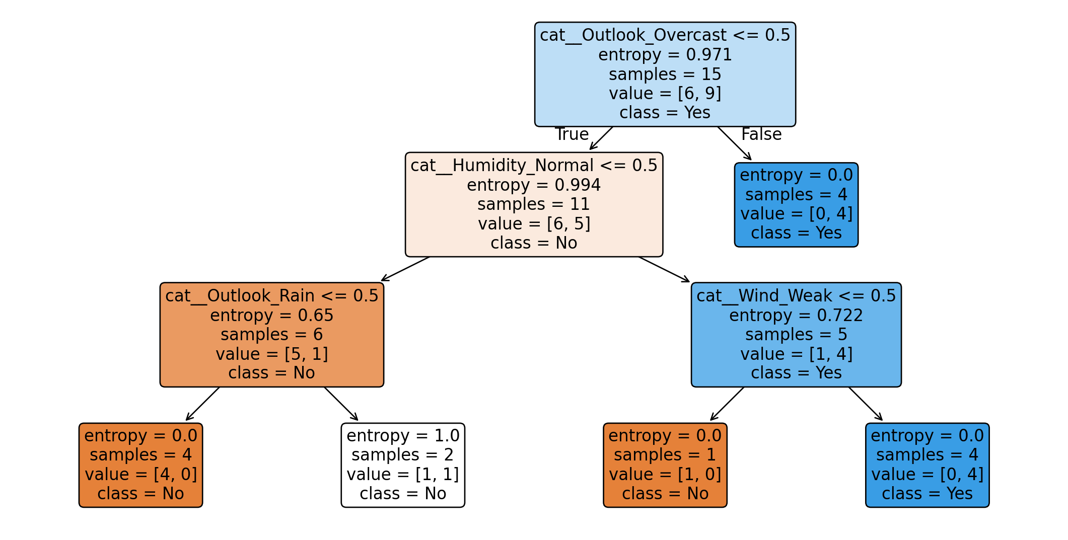
While the preceding examples computed entropy and information gain manually, production environments utilize optimized machine learning libraries. In Python, scikit-learn provides efficient decision tree implementations (Pedregosa et al. 2011).

Categorical features are typically one-hot encoded before fitting a tree configured with criterion="entropy".

from sklearn.compose import ColumnTransformer
from sklearn.preprocessing import OneHotEncoder
from sklearn.tree import DecisionTreeClassifier, plot_tree
from sklearn.pipeline import Pipeline
from sklearn.model_selection import train_test_split
from sklearn.metrics import accuracy_score, classification_report

X = df.drop(columns="Play")
y = df["Play"]

categorical_features = X.columns.tolist()

preprocess = ColumnTransformer(
    transformers=[
        ("cat", OneHotEncoder(handle_unknown="ignore"), categorical_features)
    ]
)

model = DecisionTreeClassifier(
    criterion="entropy",
    max_depth=3,
    random_state=42
)

clf = Pipeline(steps=[
    ("preprocess", preprocess),
    ("model", model)
])

clf.fit(X, y)
clf.predict(X)

array(['No', 'No', 'Yes', 'No', 'Yes', 'No', 'Yes', 'No', 'Yes', 'Yes',
       'Yes', 'Yes', 'Yes', 'No', 'No'], dtype=object)

On small datasets, evaluating performance on training data serves only as a technical sanity check. Real-world validation requires held-out test sets or cross-validation.

X_train, X_test, y_train, y_test = train_test_split(
    X, y,
    test_size=0.30,
    random_state=42,
    stratify=y
)

clf.fit(X_train, y_train)
y_pred = clf.predict(X_test)

print("Accuracy:", accuracy_score(y_test, y_pred))
print(classification_report(y_test, y_pred))

Accuracy: 0.6
              precision    recall  f1-score   support

          No       0.50      1.00      0.67         2
         Yes       1.00      0.33      0.50         3

    accuracy                           0.60         5
   macro avg       0.75      0.67      0.58         5
weighted avg       0.80      0.60      0.57         5

17 Tree Visualization

import matplotlib.pyplot as plt

clf.fit(X, y)

feature_names = clf.named_steps["preprocess"].get_feature_names_out()
tree_model = clf.named_steps["model"]

plt.figure(figsize=(14, 7))
plot_tree(
    tree_model,
    feature_names=feature_names,
    class_names=tree_model.classes_,
    filled=True,
    rounded=True
)
plt.show()

Visualizing trees allows inspecting feature usage and split points. On larger trees, visual diagrams can become unwieldy; hyperparameters such as max_depth, min_samples_split, and min_samples_leaf should be tuned to maintain model interpretability and prevent overfitting.

18 Computational Complexity

The computational complexity of tree building depends on the number of records \(n\), number of attributes \(m\), number of classes, and split evaluation costs. For categorical features, a simplified per-node split evaluation cost is \(O(mn)\).

Summing across tree levels, a balanced tree of depth \(d\) processes roughly \(n\) examples per level, yielding a total induction complexity estimate of:

\[ O(mn d), \]

where \(d\) is tree depth. In the worst case, depth can reach \(n\), incurring higher costs and producing non-generalizable unpruned trees. Continuous features require sorting or threshold scanning, modifying training complexity (Hastie et al. 2009; Pedregosa et al. 2011).

Definition. For \(n\) examples, \(m\) attributes, and tree depth \(d\), a simplified computational complexity estimate for categorical tree induction is: \[ T(n,m,d) = O(mnd). \tag{8}\]

Inference with a trained tree is highly efficient: classifying a new record requires traversing a single path from root to leaf, taking \(O(d)\) time.

19 Pros and Cons

Decision trees offer several major advantages:

• Intuitive interpretability;
• Direct extraction of human-readable rules;
• Seamless handling of both numerical and categorical variables;
• Minimal feature scaling requirements;
• Natural capture of non-linear feature interactions.

However, they also carry key limitations:

• High risk of overfitting if grown unconstrained;
• Instability and sensitivity to small training data fluctuations;
• ID3 bias toward attributes with many distinct categories;
• Standard ID3 lacks native handling of continuous numerical features;
• Greedy local optimization does not guarantee a globally optimal tree.

The greedy nature of ID3 means it selects locally optimal splits at each node without backtracking. While computationally efficient, this does not guarantee globally optimal trees. In practice, techniques like pruning, cross-validation, and ensemble methods (Random Forests, Gradient Boosting) substantially improve generalization performance (Breiman et al. 1984; Hastie et al. 2009).

20 Conclusions

Supervised classification aims to assign categorical labels to new instances based on historical observations. Decision trees offer an intuitive, interpretable framework for solving classification tasks through sequential feature tests.

Hunt’s algorithm provides the general recursive blueprint for tree construction. ID3 specifies a split selection criterion grounded in entropy and Information Gain. Entropy measures class impurity, while Information Gain quantifies impurity reduction following a split.

The baseball example illustrated how initial entropy is computed, candidate features are evaluated, root nodes selected, and branches recursively grown until pure leaves are reached. Converting trained trees into IF-THEN rules bridges the gap between quantitative predictive modeling and human explainability.

In real-world machine learning pipelines, decision trees require careful hyperparameter tuning and regularization to avoid overfitting. Nevertheless, they remain a foundational model family in data science due to their unique balance of simplicity, transparency, and competitive predictive capability.

References

Breiman, Leo, Jerome H. Friedman, Richard A. Olshen, and Charles J. Stone. 1984. Classification and Regression Trees. Wadsworth International Group.

Géron, Aurélien. 2022. Hands-on Machine Learning with Scikit-Learn, Keras, and TensorFlow. 3rd ed. O’Reilly Media.

Hastie, Trevor, Robert Tibshirani, and Jerome Friedman. 2009. The Elements of Statistical Learning: Data Mining, Inference, and Prediction. 2nd ed. Springer Series in Statistics. Springer. https://doi.org/10.1007/978-0-387-84858-7.

James, Gareth, Daniela Witten, Trevor Hastie, and Robert Tibshirani. 2021. An Introduction to Statistical Learning with Applications in R. 2nd ed. Springer Texts in Statistics. Springer. https://doi.org/10.1007/978-1-0716-1418-1.

Pedregosa, Fabian, Gaël Varoquaux, Alexandre Gramfort, et al. 2011. “Scikit-Learn: Machine Learning in Python.” Journal of Machine Learning Research 12: 2825–30. https://jmlr.org/papers/v12/pedregosa11a.html.

Quinlan, J. Ross. 1986. “Induction of Decision Trees.” Machine Learning 1 (1): 81–106. https://doi.org/10.1007/BF00116251.

Quinlan, J. Ross. 1993. C4.5: Programs for Machine Learning. Morgan Kaufmann.

Shannon, Claude E. 1948. “A Mathematical Theory of Communication.” The Bell System Technical Journal 27 (3): 379–423. https://doi.org/10.1002/j.1538-7305.1948.tb01338.x.