---
title: "CART Trees: Classification and Regression Trees"
description: "Explore CART decision trees: binary splitting rules, Gini index impurity, categorical and continuous splits, and cost-complexity pruning."
pagetitle: "CART Trees: Classification and Regression Trees"
open-graph:
description: "Explore CART decision trees: binary splitting rules, Gini index impurity, categorical and continuous splits, and cost-complexity pruning."
twitter-card:
description: "Explore CART decision trees: binary splitting rules, Gini index impurity, categorical and continuous splits, and cost-complexity pruning."
author: "Diego Villalba"
date: today
lang: en
format:
html:
toc: true
toc-depth: 3
toc-title: "Contents"
number-sections: true
code-fold: true
code-tools: true
code-summary: "Show code"
fig-align: center
theme: cosmo
highlight-style: github
smooth-scroll: true
pdf:
toc: true
toc-depth: 3
number-sections: true
documentclass: scrbook
papersize: letter
fontsize: 11pt
geometry: margin=2.5cm
keep-tex: false
execute:
echo: true
warning: false
message: false
cache: false
bibliography: [referencias_cart.bib, ../../../references.bib]
crossref:
fig-title: "Figure"
tbl-title: "Table"
eq-prefix: "Eq."
jupyter: python3
---
## Introduction
Decision trees constitute a fundamental family of supervised learning models designed to learn decision rules from labeled training data. In classification, these rules assign an observation to a categorical class label; in regression, they estimate a continuous numerical value. Within this family, the CART (*Classification and Regression Trees*) algorithm occupies a central position because it formalizes the construction of strictly binary trees capable of handling both categorical and numerical features while incorporating cost-complexity pruning mechanisms to control model complexity [@breiman1984; @hastie2009].
Unlike algorithms such as ID3, which was originally formulated for classification trees with multi-way splits on categorical features, CART builds strictly binary trees. At each internal node, the algorithm evaluates a boolean question ("does a specific condition hold?") to split data into two disjoint subsets: those meeting the condition and those that do not. The fundamental goal is selecting splits that recursively yield increasingly homogeneous child nodes with respect to the target variable.
In classification tasks, node homogeneity is measured using an impurity function. CART typically employs the Gini index, though entropy is also widely supported. In regression tasks, split criteria rely on variance reduction or Mean Squared Error (MSE) minimization. This chapter focuses primarily on CART for classification, exploring binary tree structure, Gini index calculations, categorical and continuous variable splitting rules, impurity reduction, pruning, and computational complexity.
## From Decision Trees to CART
A decision tree represents a hierarchy of conditional rules. Each internal node contains a test condition on a predictor variable, each branch represents a test outcome, and each leaf node assigns a class prediction. Classifying a new observation involves traversing the tree from root to leaf by sequentially evaluating learned branch conditions.
CART was introduced by Breiman, Friedman, Olshen, and Stone in 1984 as a unified framework for constructing classification and regression trees [@breiman1984]. Its defining features include:
- Building strictly binary trees;
- Evaluating candidate splits using formal impurity metrics;
- Handling both numerical continuous and categorical features;
- Performing greedy local split optimization at each node;
- Applying cost-complexity pruning to prevent overfitting;
- Producing highly interpretable models expressed as IF-THEN rules.
::: {.callout-note appearance="minimal"}
Definition. A CART tree is a binary decision tree where each internal node $t$ partitions dataset $D_t$ into two disjoint child subsets $D_L$ and $D_R$ using a decision rule $s$:
$$
D_t = D_L \cup D_R, \qquad D_L \cap D_R = \varnothing.
$$
:::
Binary partitioning is a key characteristic: even if a categorical feature takes more than two values, CART does not create multi-way branches. Instead, it evaluates all non-equivalent binary groupings of categories into two subsets to find the split yielding maximum purity gain.
## Classification, Purity, and Impurity
Supervised classification starts with a training set:
$$
D = \{(\mathbf{x}_i, y_i)\}_{i=1}^{n},
$$
where $\mathbf{x}_i \in \mathcal{X}$ represents predictor features for observation $i$ and $y_i \in \{1, 2, \dots, K\}$ is its target class label. The goal is learning a mapping $f: \mathcal{X} \to \{1, 2, \dots, K\}$ predicting target labels for new observations.
A node is pure if all contained observations belong to a single class, making leaf prediction unambiguous. Conversely, if a node mixes observations across multiple classes, it is impure, warranting further splits if informative candidate questions remain available.
::: {.callout-note appearance="minimal"}
Definition. Let $D_t$ be the subset of training instances reaching node $t$. The proportion of class $k$ instances in node $t$ is:
$$
p_{k,t} = \frac{1}{|D_t|}\sum_{(\mathbf{x}_i,y_i)\in D_t}\mathbf{1}(y_i=k).
$$
:::
If $p_{k,t}=1$ for some class $k$, the node is pure. As class proportions spread across multiple classes, impurity increases. This intuition is formalized by the Gini index.
## Gini Index
The Gini index measures node impurity based on class distribution. For $K$ target classes, it is defined as:
::: {.callout-note appearance="minimal"}
Definition. The Gini index of node $D_t$ with class proportions $p_{1,t},\dots,p_{K,t}$ is:
$$
Gini(D_t)=1-\sum_{k=1}^{K}p_{k,t}^{2}.
$$ {#eq-gini}
:::
This expression can be interpreted as the probability of incorrectly classifying a randomly chosen node element if it were randomly labeled according to the empirical class distribution of the node [@breiman1984; @james2021].
In binary classification with classes "Yes" and "No", if $p$ is the proportion of positive instances:
$$
Gini(D_t)=1-p^2-(1-p)^2=2p(1-p).
$$
The minimum Gini value is $0$, achieved when $p=0$ or $p=1$ (pure node). The maximum binary Gini value is $0.5$, achieved when $p=0.5$ (equal 50/50 mixture).
```{python}
import numpy as np
import pandas as pd


def gini_from_counts(counts):
    counts = np.asarray(counts, dtype=float)
    probs = counts / counts.sum()
    return 1 - np.sum(probs**2)

# Example: 9 "Yes" records and 5 "No" records
gini_raiz = gini_from_counts([9, 5])
print(f"Root Gini = {gini_raiz:.3f}")
```
In this example, initial impurity is approximately $0.459$, indicating that the root node contains a mixture of both classes.
## Evaluating Binary Splits
In CART, a split divides node dataset $D_t$ into left ($D_L$) and right ($D_R$) child subsets. Split quality is evaluated by computing the weighted average impurity of both child nodes, rather than evaluating child purity in isolation. This prevents favoring splits that isolate tiny pure nodes at the expense of overall dataset purity.
::: {.callout-note appearance="minimal"}
Definition. The weighted Gini impurity of a binary split $s$ partitioning $D_t$ into $D_L$ and $D_R$ is:
$$
Gini_s(D_t)=\frac{|D_L|}{|D_t|}Gini(D_L)+\frac{|D_R|}{|D_t|}Gini(D_R).
$$ {#eq-weighted-gini}
:::
CART selects the candidate split $s$ that minimizes weighted Gini impurity. Equivalently, this maximizes impurity reduction (Gini gain).
::: {.callout-note appearance="minimal"}
Definition. The impurity reduction achieved by split $s$ at node $D_t$ is:
$$
\Delta Gini(s,D_t)=Gini(D_t)-Gini_s(D_t).
$$ {#eq-gini-reduction}
:::
Both formulations yield identical split rankings for a given node: minimizing $Gini_s(D_t)$ is mathematically equivalent to maximizing $\Delta Gini(s,D_t)$ because parent impurity $Gini(D_t)$ is constant during evaluation.
## Binary Splits for Categorical Features
Suppose a categorical feature $A$ takes values in a finite set:
$$
\mathcal{A}=\{a_1,a_2,\dots,a_m\}.
$$
Rather than creating an $m$-way branch, CART constructs binary questions of the form:
$$
A \in S_A,
$$
where $S_A$ is a non-empty proper subset of $\mathcal{A}$. For example, if:
$$
\text{income} \in \{\text{low}, \text{medium}, \text{high}\},
$$
candidate split subsets include:
$$
\text{income} \in \{\text{low}\}, \qquad \text{income} \in \{\text{medium}\}, \qquad \text{income} \in \{\text{low}, \text{medium}\}.
$$
Each question partitions observations into two subsets: matching instances and non-matching instances.
::: {.callout-note appearance="minimal"}
Definition. For a categorical feature $A$ taking $m$ distinct categories, the number of distinct, non-trivial binary splits is:
$$
\frac{2^m-2}{2}=2^{m-1}-1.
$$ {#eq-categorical-splits}
:::
We subtract 2 because empty and full set subsets do not form valid splits. We divide by 2 because subset $S_A$ and its complement $\mathcal{A} \setminus S_A$ define the exact same physical data partition (simply swapping left and right branch assignments).
```{python}
from itertools import combinations


def binary_partitions(values):
    values = tuple(values)
    m = len(values)
    partitions = []
    seen = set()
    full = frozenset(values)
    for r in range(1, m):
        for comb in combinations(values, r):
            left = frozenset(comb)
            right = full - left
            key = frozenset([left, right])
            if key not in seen:
                seen.add(key)
                partitions.append((set(left), set(right)))
    return partitions

for left, right in binary_partitions(["low", "medium", "high"]):
    print(left, "vs", right)
```
## Binary Splits for Continuous Features
For continuous numerical features, CART evaluates candidate cut-points. For continuous feature $A$, a split takes the form:
$$
A < c \quad \text{vs.} \quad A \geq c.
$$
Standard procedure sorts unique observed values of $A$, computes midpoints between consecutive sorted values, and evaluates each midpoint as a candidate threshold $c$.
::: {.callout-note appearance="minimal"}
Definition. Given sorted unique values $a_{(1)}<a_{(2)}<\dots<a_{(r)}$ of a continuous numerical feature $A$, candidate cut-points are:
$$
c_j=\frac{a_{(j)}+a_{(j+1)}}{2}, \qquad j=1,\dots,r-1.
$$ {#eq-cutpoints}
:::
Consider the toy dataset:
$$
(20,\text{Yes}),\quad (25,\text{Yes}),\quad (30,\text{No}),\quad (40,\text{No}).
$$
Sorted values are $20, 25, 30, 40$, yielding candidate midpoints:
$$
22.5, \qquad 27.5, \qquad 35.
$$
For each threshold $c$, child subsets are formed:
$$
D_L=\{A<c\}, \qquad D_R=\{A\geq c\},
$$
and weighted Gini impurity is computed.
```{python}
import pandas as pd

edad = pd.DataFrame({
    "age": [20, 25, 30, 40],
    "target": ["Yes", "Yes", "No", "No"]
})


def gini(labels):
    counts = pd.Series(labels).value_counts().to_numpy()
    return gini_from_counts(counts)


def weighted_gini_for_cut(df, feature, target, c):
    left = df[df[feature] < c]
    right = df[df[feature] >= c]
    n = len(df)
    return (len(left)/n)*gini(left[target]) + (len(right)/n)*gini(right[target])

values = sorted(edad["age"].unique())
cuts = [(values[i] + values[i+1]) / 2 for i in range(len(values)-1)]

resultados = pd.DataFrame({
    "cutpoint": cuts,
    "weighted_gini": [weighted_gini_for_cut(edad, "age", "target", c) for c in cuts]
})
resultados
```
The optimal cut-point is $c=27.5$, producing pure child nodes (2 "Yes" on the left, 2 "No" on the right) and yielding a weighted Gini of 0.
## Complete Example: Laptop Purchase Prediction
Consider a dataset predicting whether a customer purchases a laptop computer (`buy_laptop`). Predictor features are `age`, `income`, `student`, and `credit_rating`.
```{python}
datos = pd.DataFrame({
    "id": range(1, 15),
    "age": ["youth", "youth", "middle_aged", "senior", "senior", "senior", "middle_aged", "youth", "youth", "senior", "youth", "middle_aged", "middle_aged", "senior"],
    "income": ["high", "high", "high", "medium", "low", "low", "low", "medium", "low", "medium", "medium", "medium", "high", "medium"],
    "student": ["no", "no", "no", "no", "yes", "yes", "yes", "no", "yes", "yes", "yes", "no", "yes", "no"],
    "credit_rating": ["fair", "excellent", "fair", "fair", "fair", "excellent", "excellent", "fair", "fair", "fair", "excellent", "excellent", "fair", "excellent"],
    "buy_laptop": ["no", "no", "yes", "yes", "yes", "no", "yes", "no", "yes", "yes", "yes", "yes", "yes", "no"]
})

datos
```
The target label contains 9 "yes" and 5 "no" instances, giving an initial root impurity:
```{python}
gini_inicial = gini(datos["buy_laptop"])
print(f"Initial Gini = {gini_inicial:.3f}")
```
Evaluating all non-equivalent binary partitions across categorical features:
```{python}
def weighted_gini_categorical(df, feature, target, left_values):
    left_values = set(left_values)
    left = df[df[feature].isin(left_values)]
    right = df[~df[feature].isin(left_values)]
    n = len(df)
    return (len(left)/n)*gini(left[target]) + (len(right)/n)*gini(right[target])


def best_categorical_split(df, feature, target):
    values = sorted(df[feature].unique())
    rows = []
    for left, right in binary_partitions(values):
        wg = weighted_gini_categorical(df, feature, target, left)
        rows.append({
            "feature": feature,
            "left_subset": tuple(sorted(left)),
            "right_subset": tuple(sorted(right)),
            "weighted_gini": wg,
            "gini_reduction": gini(df[target]) - wg
        })
    return pd.DataFrame(rows).sort_values("weighted_gini")

resumen = pd.concat([
    best_categorical_split(datos, col, "buy_laptop").head(1)
    for col in ["age", "income", "student", "credit_rating"]
], ignore_index=True)

resumen.sort_values("weighted_gini")
```
Here, isolating category `middle_aged` on feature `age` yields a substantial Gini reduction because all `middle_aged` records in the dataset belong to class "yes". CART recurses on child nodes until stopping criteria are met.
## Impurity Reduction and Interpretation
Gini reduction measures absolute purity improvement relative to parent node impurity. For instance, if root impurity is:
$$
Gini(D)=0.459,
$$
and a candidate split produces:
$$
Gini_s(D)=0.357,
$$
the Gini reduction is:
$$
\Delta Gini = 0.459-0.357=0.102.
$$
Higher Gini reduction signals a better split. CART systematically tests all available feature splits at a node, selecting the one with maximum impurity reduction, and repeats this process recursively on each child node.
## Stopping Criteria
Trees cannot grow indefinitely without overfitting. Partitioning stops when any of the following conditions are met:
- The current node is completely pure ($Gini = 0$);
- No remaining predictor features are available for splitting;
- The number of instances in the node falls below a minimum threshold (`min_samples_split`);
- Gini reduction falls below a specified minimum improvement threshold;
- Maximum tree depth (`max_depth`) has been reached;
- All candidate splits yield invalid or redundant partitions.
Stopping rules play a critical role: unconstrained trees memorize training noise, ruining generalization performance.
## Cost-Complexity Pruning
A key architectural feature of CART is cost-complexity pruning. The tree is initially allowed to grow deep, after which weak branches providing minimal predictive gain relative to tree complexity are pruned [@breiman1984].
For tree $T$, cost-complexity objective combines empirical error with a complexity penalty:
::: {.callout-note appearance="minimal"}
Definition. The cost-complexity criterion for tree $T$ parameterized by $\alpha \geq 0$ is:
$$
R_{\alpha}(T)=R(T)+\alpha |T|,
$$ {#eq-cost-complexity}
:::
where $R(T)$ is empirical training error, $|T|$ is the number of terminal leaf nodes, and $\alpha \ge 0$ controls complexity penalty. Setting $\alpha=0$ keeps the unpruned full tree. Larger $\alpha$ values favor smaller, simpler trees.
Pruning yields simpler, more interpretable models less prone to overfitting. In `scikit-learn`, cost-complexity pruning is configured via `ccp_alpha` [@pedregosa2011].
```{python}
from sklearn.tree import DecisionTreeClassifier, plot_tree
from sklearn.compose import ColumnTransformer
from sklearn.preprocessing import OneHotEncoder
from sklearn.pipeline import Pipeline
from sklearn.model_selection import train_test_split
from sklearn.metrics import accuracy_score

X = datos[["age", "income", "student", "credit_rating"]]
y = datos["buy_laptop"]

preprocess = ColumnTransformer(
    transformers=[("cat", OneHotEncoder(handle_unknown="ignore"), X.columns)]
)

modelo = Pipeline(steps=[
    ("preprocess", preprocess),
    ("tree", DecisionTreeClassifier(criterion="gini", random_state=42))
])

modelo.fit(X, y)
pred = modelo.predict(X)
print(f"Training Accuracy = {accuracy_score(y, pred):.3f}")
```
## Visualizing a Trained Tree
```{python}
import matplotlib.pyplot as plt

modelo_simple = Pipeline(steps=[
    ("preprocess", preprocess),
    ("tree", DecisionTreeClassifier(
        criterion="gini",
        max_depth=3,
        random_state=42
    ))
])
modelo_simple.fit(X, y)

feature_names = modelo_simple.named_steps["preprocess"].get_feature_names_out()

plt.figure(figsize=(14, 6))
plot_tree(
    modelo_simple.named_steps["tree"],
    feature_names=feature_names,
    class_names=modelo_simple.named_steps["tree"].classes_,
    filled=True,
    rounded=True
)
plt.show()
```
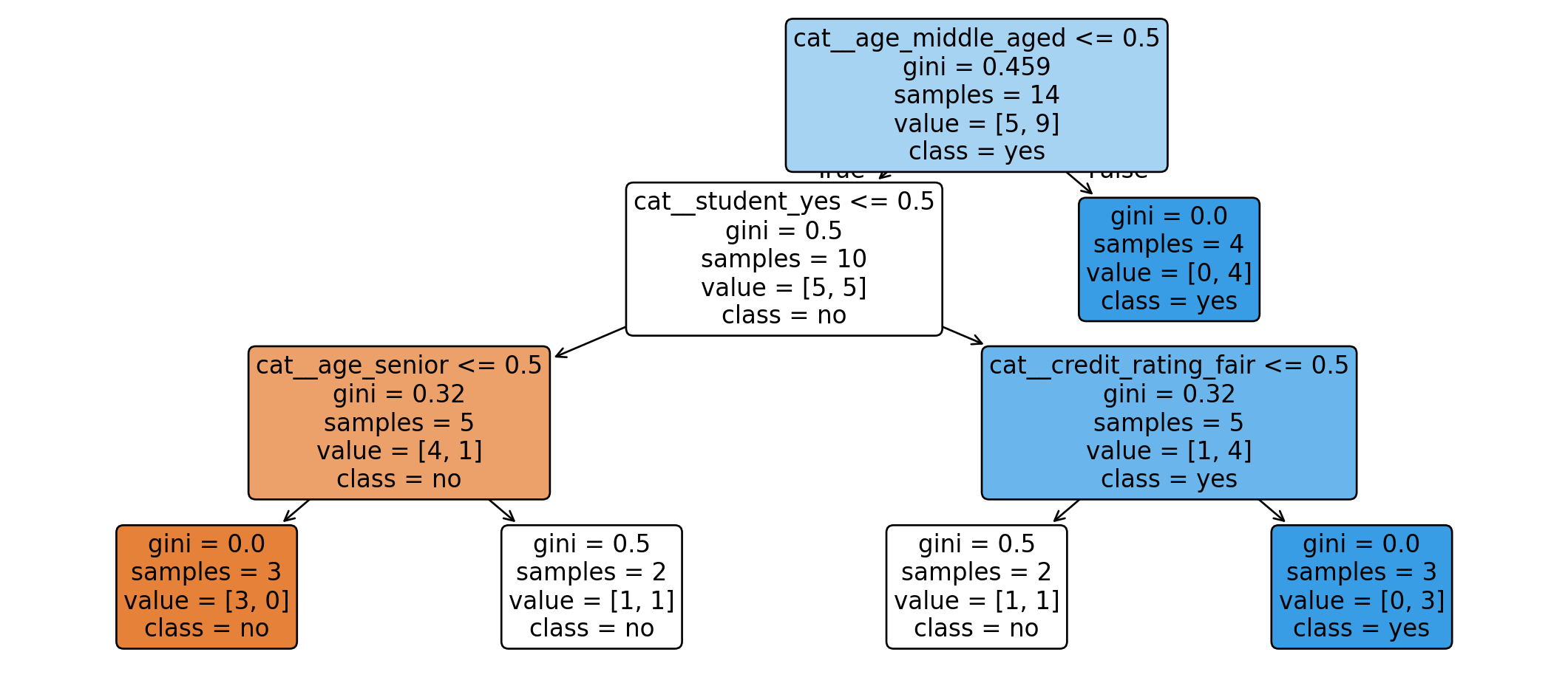
Visualizing decision trees enables inspecting learned split conditions, node impurities, and leaf class distributions. Interpretability remains a chief advantage of decision trees over black-box models.
## Extracting Classification Rules
Trees translate directly into IF-THEN rules. Each root-to-leaf path forms a single rule. For example:
$$
\text{IF age} \neq \text{middle\_aged AND student} = \text{yes THEN buy\_laptop} = \text{yes}.
$$
Extracted rules make model logic transparent to non-technical stakeholders, allowing auditability for bias or counter-intuitive logic.
```{python}
from sklearn.tree import export_text

arbol = modelo_simple.named_steps["tree"]
reglas = export_text(arbol, feature_names=list(feature_names))
print(reglas)
```
## CART for Regression
While this chapter focuses on classification, CART applies equally to regression tasks. For regression trees, leaf nodes predict continuous numerical values (typically node mean target values).
Split selection in regression minimizes node variance or Residual Sum of Squares (RSS):
::: {.callout-note appearance="minimal"}
Definition. In a regression tree, for split $s$ partitioning $D_t$ into $D_L$ and $D_R$, RSS error is:
$$
RSS(s)=\sum_{i\in D_L}(y_i-\bar{y}_L)^2+\sum_{i\in D_R}(y_i-\bar{y}_R)^2.
$$ {#eq-rss-cart}
:::
Thus, CART unifies classification and regression under a common framework: recursively partitioning feature space into internally homogeneous regions.
## Computational Complexity
CART training complexity depends on sample size $n$, feature count $m$, feature types, and final tree depth. For numerical features, sorting values at each node takes $O(mn \log n)$ initial time.
Overall training complexity for balanced binary trees can be estimated as:
$$
O(mn\log n).
$$
Factors influencing complexity:
- $n$ dictates training instance evaluation counts;
- $m$ dictates feature evaluations per split;
- Tree depth dictates partitioning iterations;
- Categorical features with many categories scale as $2^{m-1}-1$ candidate binary splits.
Hyperparameters like `max_depth`, `min_samples_split`, and `ccp_alpha` keep computational and structural complexity in check.
## Pros and Cons
CART offers significant benefits:
- Highly interpretable, self-explanatory rules;
- Minimal data scaling / normalization required;
- Naturally captures non-linear feature interactions;
- Unified framework for classification and regression;
- Serves as the foundational base learner for Random Forests and Gradient Boosted Trees [@breiman2001; @friedman2001greedy].
Key limitations include:
- High susceptibility to overfitting if unregularized;
- Instability: small data perturbations produce different tree structures;
- Greedy local optimization does not guarantee global optimal trees;
- Single decision trees generally underperform ensemble methods;
- High-cardinality categorical features can create complex, unstable splits.
## Conclusions
CART is a cornerstone decision tree algorithm. Its core mechanic is recursively partitioning feature space using binary splits to minimize node impurity. In classification, the Gini index provides an effective impurity measure; in regression, RSS minimization guides partitioning.
The CART framework combines interpretability, versatility, and mathematical clarity. Impurity-weighted split selection, Gini gain maximization, and cost-complexity pruning allow building accurate models while controlling overfitting. Beyond its standalone utility, CART provides the essential foundation for state-of-the-art ensemble techniques across modern data science.
## References {.unnumbered}
::: {#refs}
:::