41  Evaluating a Classification Model

42 Evaluating a Classification Model

42.1 Introduction

Model evaluation is a central phase of supervised classification. In classification tasks, a dataset is available where both predictor variables and ground-truth target labels are known for every instance. From these observations, the goal is to learn a decision rule capable of assigning correct class labels to unseen future data (Hastie et al. 2009; James et al. 2021).

In practical terms, evaluating a classifier goes far beyond counting correct predictions. Model quality depends on how errors are distributed, class balance, relative costs of false positives and false negatives, and operational context. For example, in a spam filter, allowing a few unsolicited emails into the primary inbox may be tolerable, but incorrectly sending an urgent email to the spam folder is a severe error. In medical diagnostics, conversely, generating false positives is far preferable to missing true cases of disease (Fawcett 2006; Saito and Rehmsmeier 2015).

This chapter establishes the core concepts required to evaluate classification models. First, we examine data partitioning methods such as holdout and \(K\)-fold cross-validation. Next, we introduce the confusion matrix and key metrics derived from it: accuracy, error rate, precision, recall, sensitivity, specificity, and F1-score. Finally, we explore the ROC curve, Area Under the Curve (AUC), and metric selection strategies suited to specific problem constraints.

42.2 Supervised Learning and Evaluation

Supervised learning operates on labeled datasets. Each observation contains a feature vector \(\mathbf{x}_i\) and an associated target class \(y_i\). In binary classification, \(y_i \in \{0, 1\}\), where \(1\) denotes the positive class and \(0\) denotes the negative class.

Definition. A supervised dataset is a collection of input-output pairs: \[ \mathcal{D} = \{(\mathbf{x}_i, y_i)\}_{i=1}^{n}, \qquad \mathbf{x}_i \in \mathbb{R}^p,\quad y_i \in \mathcal{Y} \]

A classification model can be conceptualized as a trainable function: \[ f_\theta:\mathbb{R}^p \to \mathcal{Y}, \] where \(\theta\) represents parameters learned from data. In probabilistic models, the classifier outputs estimated probabilities or confidence scores: \[ \hat{p}_i = P_\theta(y_i = 1 \mid \mathbf{x}_i). \] Converting continuous scores into discrete class assignments requires a decision threshold \(\tau\): \[ \hat{y}_i = \begin{cases} 1, & \hat{p}_i \geq \tau,\\ 0, & \hat{p}_i < \tau. \end{cases} \]

Evaluation must be performed on data withheld during training to reliably estimate generalization performance on unseen instances. Evaluating a model solely on its training set yields overly optimistic estimates due to overfitting (Hastie et al. 2009; Bishop 2006).

42.3 Data Partitioning

Standard methodology splits datasets into disjoint subsets with distinct operational roles: training, validation, and testing.

Definition. A train-validation-test split partitions dataset \(\mathcal{D}\) into three pairwise disjoint subsets: \[ \mathcal{D} = \mathcal{D}_{\text{train}} \cup \mathcal{D}_{\text{val}} \cup \mathcal{D}_{\text{test}}, \qquad \mathcal{D}_{a} \cap \mathcal{D}_{b} = \varnothing \quad (a \neq b) \]

The training set fits model parameters. The validation set compares hyperparameter configurations and selects candidate models. The test set remains strictly untouched until final evaluation to provide an unbiased estimate of generalization capability.

A typical split distribution:

Subset	Typical Ratio	Primary Function
Training	70 %	Fit model parameters
Validation	15 %	Tune hyperparameters & select model
Testing	15 %	Estimate final generalization performance

Alternatively, a 50 % train / 25 % validation / 25 % test split is used when higher validation and testing stability is required. Choice of split ratio depends on overall dataset size, computational cost, and expected evaluation variance.

42.3.1 Holdout Method

The holdout method partitions a dataset a single time into static subsets (e.g., 80 % training and 20 % testing).

Definition. The holdout method constructs a single partition: \[ \mathcal{D} = \mathcal{D}_{\text{train}} \cup \mathcal{D}_{\text{test}}, \qquad \mathcal{D}_{\text{train}} \cap \mathcal{D}_{\text{test}} = \varnothing \]

Its primary advantage is computational simplicity and speed, making it scalable to massive datasets. Its primary limitation is high variance: evaluation results depend heavily on the specific random split. If the test set happens to contain disproportionately easy cases, reported performance will be artificially high; if it contains unusually hard cases, performance will appear artificially poor.

Under class imbalance, unstratified holdout risks creating test sets with insufficient representation of the minority class. For example, in a dataset with 950 healthy and 50 diseased records, random splitting might place almost no positive cases in test sets, rendering metrics like recall highly unstable.

42.3.2 Stratified Random Sampling

Stratified sampling mitigates unrepresentative split risks by preserving overall class proportions within each subset. If class A makes up 80 % of the dataset and class B makes up 20 %, training, validation, and test subsets maintain matching 80/20 proportions.

Definition. A stratified partition preserves marginal class distributions across subsets: \[ P_{\mathcal{D}_{\text{train}}}(Y=y) \approx P_{\mathcal{D}_{\text{val}}}(Y=y) \approx P_{\mathcal{D}_{\text{test}}}(Y=y) \approx P_{\mathcal{D}}(Y=y) \]

Stratification is essential under class imbalance. However, while preserving proportions, single stratified splits can still suffer from sample variance on small datasets.

42.3.3 Repeated Holdout

Repeated holdout performs multiple independent random splits and averages evaluated metrics across runs, smoothing out single-split variance.

Definition. In repeated holdout, \(R\) independent partitions are generated and metric \(M\) is reported as the mean across runs: \[ \bar{M} = \frac{1}{R} \sum_{r=1}^{R} M^{(r)} \]

For example, if 5 repetitions yield accuracy scores of 85 %, 82 %, 88 %, 84 %, and 86 %, the mean holdout accuracy is: \[ \bar{M} = \frac{85 + 82 + 88 + 84 + 86}{5} = 85\%. \]

While more reliable than single holdout, repeated holdout can overlap test instances across runs. For small datasets, \(K\)-fold cross-validation provides a more systematic approach.

42.3.4 K-fold Cross-Validation

\(K\)-fold cross-validation partitions data into \(K\) equal-sized folds. The model is trained \(K\) times: in each iteration \(k\), fold \(k\) serves as the test set while the remaining \(K-1\) folds serve as training data (Stone 1974; Kohavi 1995).

Definition. In \(K\)-fold cross-validation, overall metric \(M\) is estimated as the mean score across all \(K\) test folds: \[ \widehat{M}_{\text{CV}} = \frac{1}{K} \sum_{k=1}^{K} M_k \]

For instance, with \(K=5\), each fold contains 20 % of data. Iteration 1 evaluates on fold 1 while training on folds 2–5; iteration 2 evaluates on fold 2 while training on folds 1, 3, 4, 5; and so forth.

If test fold accuracy scores are 82 %, 80 %, 84 %, 81 %, and 83 %, the 5-fold cross-validation accuracy is: \[ \widehat{M}_{\text{CV}} = \frac{82 + 80 + 84 + 81 + 83}{5} = 82\%. \]

Cross-validation maximizes data utilization because every observation is evaluated in a test fold exactly once and used for training in \(K-1\) folds. Its primary cost is computational (\(K\) training passes). In practice, \(K=5\) or \(K=10\) are standard choices (Kohavi 1995).

42.4 Python Example: Holdout and Cross-Validation

The following Python example uses scikit-learn to fit a Logistic Regression classifier on a synthetic binary problem, comparing stratified holdout and 5-fold cross-validation.

import numpy as np
from sklearn.datasets import make_classification
from sklearn.model_selection import train_test_split, StratifiedKFold, cross_validate
from sklearn.linear_model import LogisticRegression
from sklearn.metrics import accuracy_score, precision_score, recall_score, f1_score

X, y = make_classification(
    n_samples=1000,
    n_features=10,
    n_informative=5,
    n_redundant=2,
    weights=[0.85, 0.15],
    random_state=42
)

X_train, X_test, y_train, y_test = train_test_split(
    X,
    y,
    test_size=0.20,
    stratify=y,
    random_state=42
)

model = LogisticRegression(max_iter=1000)
model.fit(X_train, y_train)

y_pred = model.predict(X_test)

metricas_holdout = {
    "accuracy": accuracy_score(y_test, y_pred),
    "precision": precision_score(y_test, y_pred),
    "recall": recall_score(y_test, y_pred),
    "f1": f1_score(y_test, y_pred),
}

metricas_holdout

{'accuracy': 0.87,
 'precision': 0.7777777777777778,
 'recall': 0.22580645161290322,
 'f1': 0.35}

cv = StratifiedKFold(n_splits=5, shuffle=True, random_state=42)

scores = cross_validate(
    model,
    X,
    y,
    cv=cv,
    scoring=["accuracy", "precision", "recall", "f1"],
    return_train_score=False
)

{metrica: scores[f"test_{metrica}"].mean()
 for metrica in ["accuracy", "precision", "recall", "f1"]}

{'accuracy': np.float64(0.859),
 'precision': np.float64(0.5909090909090909),
 'recall': np.float64(0.29290322580645156),
 'f1': np.float64(0.3833043294837315)}

This example highlights why accuracy alone is insufficient: on imbalanced data, high accuracy can be achieved simply by favoring the majority class while missing positive cases (low recall).

42.5 Confusion Matrix

The confusion matrix cross-tabulates actual ground-truth labels against model predictions. In binary classification, it tracks four counts: true positives, true negatives, false positives, and false negatives.

Definition. For positive class \(1\) and negative class \(0\), the confusion matrix is structured as: \[ \begin{array}{c|cc} & \hat{y}=0 & \hat{y}=1\\ \hline y=0 & TN & FP\\ y=1 & FN & TP \end{array} \]

Count interpretations:

Symbol	Name	Description
\(TP\)	True Positive	Actual positive correctly predicted as positive
\(TN\)	True Negative	Actual negative correctly predicted as negative
\(FP\)	False Positive	Actual negative incorrectly predicted as positive
\(FN\)	False Negative	Actual positive incorrectly predicted as negative

In spam filtering, a false positive occurs when legitimate email is misclassified as spam. A false negative occurs when spam bypasses the filter into the main inbox.

42.6 Basic Classification Metrics

From the confusion matrix, several complementary performance metrics are derived:

42.6.1 Accuracy and Error Rate

Definition. Accuracy is the overall proportion of correct predictions: \[ \text{Accuracy} = \frac{TP + TN}{TP + TN + FP + FN} \]

Accuracy measures overall correctness. It is informative when classes are balanced and error costs are equal.

Definition. Error rate is the overall proportion of incorrect predictions: \[ \text{Error Rate} = \frac{FP + FN}{TP + TN + FP + FN} = 1 - \text{Accuracy} \]

42.6.2 Precision

Definition. Precision measures the proportion of positive predictions that are correct: \[ \text{Precision} = \frac{TP}{TP + FP} \]

Precision evaluates positive prediction reliability. High precision is crucial when false positives carry significant costs (e.g., fraudulent transaction blocking).

42.6.3 Recall, Sensitivity, and True Positive Rate

Definition. Recall (Sensitivity or True Positive Rate) measures the proportion of actual positive cases successfully detected: \[ \text{Recall} = \text{Sensitivity} = \text{TPR} = \frac{TP}{TP + FN} \]

Recall measures positive case coverage. It is paramount when false negatives carry severe consequences (e.g., medical diagnostics).

42.6.4 Specificity and False Positive Rate

Definition. Specificity (True Negative Rate) measures the proportion of actual negative cases correctly identified: \[ \text{Specificity} = \frac{TN}{TN + FP} \]

Definition. False Positive Rate (FPR) measures the proportion of actual negative cases incorrectly flagged as positive: \[ \text{FPR} = \frac{FP}{FP + TN} = 1 - \text{Specificity} \]

42.6.5 F1-Score

Definition. The F1-score is the harmonic mean of precision and recall: \[ F_1 = 2 \cdot \frac{\text{Precision}\cdot \text{Recall}} {\text{Precision} + \text{Recall}} \]

F1-score provides a single metric balancing precision and recall, heavily penalizing extreme trade-offs. It is particularly effective for evaluating imbalanced classification tasks (Sokolova and Lapalme 2009).

42.6.6 Balanced Accuracy

Definition. Balanced Accuracy is the arithmetic mean of sensitivity and specificity: \[ \text{Balanced Accuracy} = \frac{\text{Sensitivity} + \text{Specificity}}{2} \]

Balanced accuracy prevents majority-class dominance from masking poor minority-class performance under class imbalance.

42.7 Python Example: Confusion Matrix and Metrics

from sklearn.metrics import confusion_matrix, classification_report

cm = confusion_matrix(y_test, y_pred)
cm

array([[167,   2],
       [ 24,   7]])

print(classification_report(y_test, y_pred, target_names=["Class 0", "Class 1"]))

              precision    recall  f1-score   support

     Class 0       0.87      0.99      0.93       169
     Class 1       0.78      0.23      0.35        31

    accuracy                           0.87       200
   macro avg       0.83      0.61      0.64       200
weighted avg       0.86      0.87      0.84       200

Computing metrics manually from confusion matrix components:

tn, fp, fn, tp = cm.ravel()

accuracy = (tp + tn) / (tp + tn + fp + fn)
error_rate = (fp + fn) / (tp + tn + fp + fn)
precision = tp / (tp + fp)
recall = tp / (tp + fn)
specificity = tn / (tn + fp)
f1 = 2 * precision * recall / (precision + recall)
balanced_accuracy = (recall + specificity) / 2

{
    "accuracy": accuracy,
    "error_rate": error_rate,
    "precision": precision,
    "recall": recall,
    "specificity": specificity,
    "f1": f1,
    "balanced_accuracy": balanced_accuracy,
}

{'accuracy': np.float64(0.87),
 'error_rate': np.float64(0.13),
 'precision': np.float64(0.7777777777777778),
 'recall': np.float64(0.22580645161290322),
 'specificity': np.float64(0.9881656804733728),
 'f1': np.float64(0.35000000000000003),
 'balanced_accuracy': np.float64(0.606986066043138)}

42.8 Metric Selection Guidelines

Metric selection depends on domain goals and relative error costs:

Metric	Primary Use Case	Key Decision Question
Accuracy	Balanced classes, equal error costs	Are all classification errors equally costly?
Error rate	Overall error percentage tracking	What overall failure rate is acceptable?
Precision	Minimizing False Positives	When the model predicts positive, how reliable is it?
Recall / Sensitivity	Minimizing False Negatives	How many true positive cases can we afford to miss?
Specificity	Minimizing False Alarms on Negatives	How effectively are true negative cases preserved?
F1-score	Imbalanced classes, balancing P & R	Is there a direct trade-off between FP and FN costs?

Consider medical cancer screening models:

Model	TPR	FPR
Model A	0.92	0.35
Model B	0.81	0.08

Model A captures more true cancers (high sensitivity) at the expense of higher false alarms. In initial screening, Model A may be preferred to avoid missed diagnoses. However, if follow-up biopsies carry high physical or financial costs, Model B offers a cleaner balance. Metric selection must align with operational domain realities (Fawcett 2006).

42.9 Decision Thresholds

Probabilistic models output continuous confidence scores \(\hat{p}(\mathbf{x}) \in [0, 1]\). Converting scores into class predictions depends on decision threshold \(\tau\).

Definition. Given probability score \(\hat{p}(\mathbf{x})\), a binary decision rule with threshold \(\tau\) is: \[ \hat{y}(\mathbf{x};\tau) = \mathbb{I}\{\hat{p}(\mathbf{x}) \geq \tau\} \]

Lowering \(\tau\) from 0.70 to 0.30 classifies more instances as positive. This raises TPR (catching more positive cases) while simultaneously raising FPR (generating more false alarms).

from sklearn.metrics import confusion_matrix

probs = model.predict_proba(X_test)[:, 1]

for tau in [0.70, 0.50, 0.30]:
    y_pred_tau = (probs >= tau).astype(int)
    tn, fp, fn, tp = confusion_matrix(y_test, y_pred_tau).ravel()
    tpr = tp / (tp + fn)
    fpr = fp / (fp + tn)
    print(f"threshold={tau:.2f} | TPR={tpr:.3f} | FPR={fpr:.3f}")

threshold=0.70 | TPR=0.129 | FPR=0.000
threshold=0.50 | TPR=0.226 | FPR=0.012
threshold=0.30 | TPR=0.613 | FPR=0.041

42.10 ROC Curve and AUC

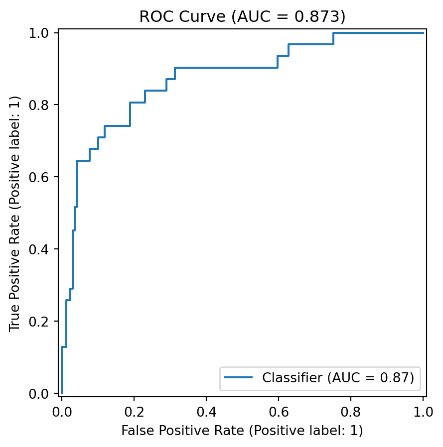
The ROC curve evaluates classifier trade-offs across all decision thresholds by plotting True Positive Rate vs. False Positive Rate (Fawcett 2006).

Definition. The ROC curve is the parametric set of points: \[ \text{ROC} = \left\{ \left( \text{FPR}(\tau), \text{TPR}(\tau) \right) : \tau \in \mathbb{R} \right\} \]

An ideal classifier hugs the top-left corner (\(\text{TPR}=1, \text{FPR}=0\)). The diagonal line represents random guessing.

AUC summarizes the area under the ROC curve into a single scalar, representing the probability that a randomly chosen positive instance receives a higher prediction score than a randomly chosen negative instance (Fawcett 2006).

Definition. Area Under the ROC Curve (AUC) is: \[ \text{AUC} = \int_{0}^{1} \text{TPR}(\text{FPR})\,d(\text{FPR}) \]

General AUC guidelines:

AUC Range	General Interpretation
0.90–1.00	Outstanding
0.80–0.90	Good / Excellent
0.70–0.80	Acceptable
0.60–0.70	Poor
0.50–0.60	No discriminative value

High AUC does not guarantee optimal performance at a specific operational threshold. Furthermore, under severe class imbalance, Precision–Recall curves offer superior analytical insight (Saito and Rehmsmeier 2015).

42.11 Python Example: ROC Curve and AUC

import matplotlib.pyplot as plt
from sklearn.metrics import RocCurveDisplay, roc_auc_score

auc = roc_auc_score(y_test, probs)

RocCurveDisplay.from_predictions(y_test, probs)
plt.title(f"ROC Curve (AUC = {auc:.3f})")
plt.show()

42.12 Precision–Recall Curves

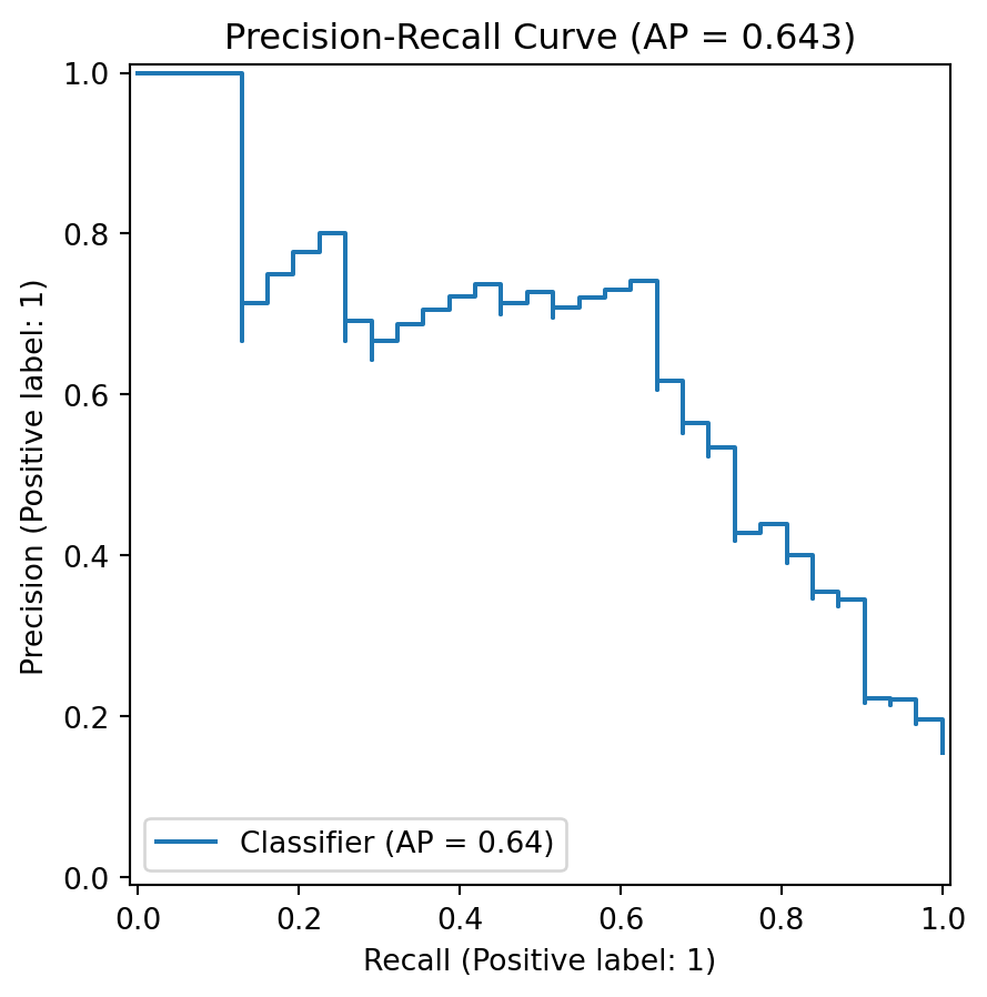
When the positive class is rare, ROC curves can present overly optimistic performance views. Precision–Recall curves evaluate positive class recovery without True Negative domination (Saito and Rehmsmeier 2015).

Definition. The Precision–Recall curve plots: \[ \text{PR} = \left\{ \left( \text{Recall}(\tau), \text{Precision}(\tau) \right) : \tau \in \mathbb{R} \right\} \]

from sklearn.metrics import PrecisionRecallDisplay, average_precision_score

ap = average_precision_score(y_test, probs)

PrecisionRecallDisplay.from_predictions(y_test, probs)
plt.title(f"Precision-Recall Curve (AP = {ap:.3f})")
plt.show()

Average Precision (AP) computes weighted precision across recall increments. Unlike ROC-AUC, its baseline equals positive class prevalence.

42.13 Recommended Classifier Evaluation Workflow

A reproducible evaluation pipeline follows these steps:

1. Formally define the target positive class and operational goal.
2. Reserve a test set before hyperparameter tuning.
3. Apply stratified partitioning under class imbalance.
4. Fit candidate models on training data.
5. Tune hyperparameters using cross-validation.
6. Evaluate the selected model once on the held-out test set.
7. Report confusion matrices and domain-aligned metrics.
8. Tune decision thresholds for continuous probability outputs.
9. Fully document random seeds, split protocols, and library versions.

42.14 Full Python Evaluation Example

from sklearn.metrics import (
    accuracy_score,
    balanced_accuracy_score,
    precision_score,
    recall_score,
    f1_score,
    roc_auc_score,
    confusion_matrix,
)

def evaluar_clasificador(y_true, y_score, threshold=0.5):
    y_pred = (y_score >= threshold).astype(int)

    tn, fp, fn, tp = confusion_matrix(y_true, y_pred).ravel()

    return {
        "threshold": threshold,
        "TP": tp,
        "TN": tn,
        "FP": fp,
        "FN": fn,
        "accuracy": accuracy_score(y_true, y_pred),
        "balanced_accuracy": balanced_accuracy_score(y_true, y_pred),
        "precision": precision_score(y_true, y_pred, zero_division=0),
        "recall": recall_score(y_true, y_pred),
        "specificity": tn / (tn + fp),
        "f1": f1_score(y_true, y_pred),
        "auc": roc_auc_score(y_true, y_score),
    }

for tau in [0.3, 0.5, 0.7]:
    print(evaluar_clasificador(y_test, probs, threshold=tau))

{'threshold': 0.3, 'TP': np.int64(19), 'TN': np.int64(162), 'FP': np.int64(7), 'FN': np.int64(12), 'accuracy': 0.905, 'balanced_accuracy': np.float64(0.7857415537316281), 'precision': 0.7307692307692307, 'recall': 0.6129032258064516, 'specificity': np.float64(0.9585798816568047), 'f1': 0.6666666666666666, 'auc': np.float64(0.872876503149456)}
{'threshold': 0.5, 'TP': np.int64(7), 'TN': np.int64(167), 'FP': np.int64(2), 'FN': np.int64(24), 'accuracy': 0.87, 'balanced_accuracy': np.float64(0.606986066043138), 'precision': 0.7777777777777778, 'recall': 0.22580645161290322, 'specificity': np.float64(0.9881656804733728), 'f1': 0.35, 'auc': np.float64(0.872876503149456)}
{'threshold': 0.7, 'TP': np.int64(4), 'TN': np.int64(169), 'FP': np.int64(0), 'FN': np.int64(27), 'accuracy': 0.865, 'balanced_accuracy': np.float64(0.564516129032258), 'precision': 1.0, 'recall': 0.12903225806451613, 'specificity': np.float64(1.0), 'f1': 0.22857142857142856, 'auc': np.float64(0.872876503149456)}

42.15 Conclusions

Evaluating classification models requires moving beyond simple accuracy calculations. Proper data partitioning ensures reliable generalization estimates. Holdout splits are fast but can suffer from split variance. \(K\)-fold cross-validation provides robust, low-variance estimates at higher computational cost.

The confusion matrix provides the foundation for derived performance metrics: precision, recall, specificity, F1-score, and balanced accuracy. Each metric evaluates distinct performance aspects and must be aligned with domain error costs. High sensitivity minimizes missed positive cases in screening; high precision minimizes false alarms in fraud detection.

Finally, ROC and Precision–Recall curves analyze model performance across all thresholds, enabling threshold selection tailored to specific operational requirements.

References

Bishop, Christopher M. 2006. Pattern Recognition and Machine Learning. Information Science and Statistics. Springer.

Fawcett, Tom. 2006. “An Introduction to ROC Analysis.” Pattern Recognition Letters 27 (8): 861–74. https://doi.org/10.1016/j.patrec.2005.10.010.

Hastie, Trevor, Robert Tibshirani, and Jerome Friedman. 2009. The Elements of Statistical Learning: Data Mining, Inference, and Prediction. 2nd ed. Springer Series in Statistics. Springer. https://doi.org/10.1007/978-0-387-84858-7.

James, Gareth, Daniela Witten, Trevor Hastie, and Robert Tibshirani. 2021. An Introduction to Statistical Learning with Applications in R. 2nd ed. Springer Texts in Statistics. Springer. https://doi.org/10.1007/978-1-0716-1418-1.

Kohavi, Ron. 1995. “A Study of Cross-Validation and Bootstrap for Accuracy Estimation and Model Selection.” Proceedings of the 14th International Joint Conference on Artificial Intelligence (IJCAI) 2: 1137–43.

Saito, Takaya, and Marc Rehmsmeier. 2015. “The Precision-Recall Plot Is More Informative Than the ROC Plot When Evaluating Binary Classifiers on Imbalanced Datasets.” PLOS ONE 10 (3): e0118432. https://doi.org/10.1371/journal.pone.0118432.

Sokolova, Marina, and Guy Lapalme. 2009. “A Systematic Analysis of Performance Measures for Classification Tasks.” Information Processing & Management 45 (4): 427–37. https://doi.org/10.1016/j.ipm.2009.03.002.

Stone, Mervyn. 1974. “Cross-Validatory Choice and Assessment of Statistical Predictions.” Journal of the Royal Statistical Society: Series B 36 (2): 111–47. https://doi.org/10.1111/j.2517-6161.1974.tb00994.x.