flowchart TB

    %% ----- Subgraphs -----
    subgraph Sources
        A1[Student Information System]
        A2[Admissions System]
        A3[Financial System]
        A4[Human Resources System]
        A5[Surveys / CSV Files]
    end

    subgraph ETL
        B1[Extraction]
        B2[Cleaning]
        B3[Transformation]
        B4[Integration]
    end

    subgraph DW["Academic Data Warehouse"]
        C1[(Evaluation Fact Table)]
        C2[(Student Dimension)]
        C3[(Course Dimension)]
        C4[(Time Dimension)]
        C5[(Faculty Dimension)]
    end

    subgraph Analytics
        D1[Academic Data Mart]
        D2[Performance Dashboard]
        D3[Cohort Analysis]
        D4[Attrition Report]
    end

    %% ----- Flow -----
    A1 --> B1
    A2 --> B1
    A3 --> B1
    A4 --> B1
    A5 --> B1

    B1 --> B2 --> B3 --> B4

    B4 --> C1
    B4 --> C2
    B4 --> C3
    B4 --> C4
    B4 --> C5

    C1 --> D1
    D1 --> D2
    D1 --> D3
    D1 --> D4

    %% ----- Styles -----
    classDef fuentes fill:#e8f0fe,stroke:#2b5dab,stroke-width:1px,color:#000;
    classDef etl fill:#fff3e0,stroke:#e65100,stroke-width:1px,color:#000;
    classDef dw fill:#e8f5e9,stroke:#1b5e20,stroke-width:1px,color:#000;
    classDef analitica fill:#f3e5f5,stroke:#6a1b9a,stroke-width:1px,color:#000;

    class A1,A2,A3,A4,A5 fuentes;
    class B1,B2,B3,B4 etl;
    class C1,C2,C3,C4,C5 dw;
    class D1,D2,D3,D4 analitica;
5 Data Warehouse
5.1 Data for Decision Making
Modern organizations generate vast volumes of data daily: sales, financial transactions, academic records, medical consultations, and digital interactions.
However, operating a business is fundamentally different from analyzing it. Operational systems are engineered to log transactions efficiently, not to answer strategic questions.
For instance:
- A sales system records individual purchases.
- But answering questions like:
- Which product sold the most over the past year?
- How have sales evolved over the last five years?
- Which store branch exhibits top performance?
requires a distinct structure optimized for historical analysis, aggregation, and temporal comparisons.
The difference represents a shift in perspective: operational systems observe each event as it occurs, while a Data Warehouse gathers those events to explain how the business changes over time. The former answers “what just happened?”; the latter helps answer “what pattern is emerging, and what decision should be taken?”.
Daily Operations
Sales, enrollments, payments, consultations, and individual events.
Question: What just happened?
Data Warehouse
Integrates sources, standardizes definitions, and preserves a queryable historical memory.
Function: Convert disparate events into context.
Informed Decision
Trends, comparisons, KPIs, alerts, and shared domain insights.
Question: What should we do?
Conceptual Diagram: The Data Warehouse acts as a bridge between daily operations and decision-making.
In this context, data analysis does not begin with technology, but with a clear definition of the business problem. One of the most widely used frameworks to structure this process is CRISP-DM (Cross Industry Standard Process for Data Mining).
CRISP-DM proposes a systematic framework consisting of six phases:
- Business Understanding: Identify strategic goals and translate them into analytical questions.
- Data Understanding: Explore available data sources, evaluate quality, and detect inconsistencies.
- Data Preparation: Clean, transform, and integrate information.
- Modeling: Apply analytical techniques or statistical models.
- Evaluation: Verify whether results meet the original business objectives.
- Deployment: Implement findings into operations or decision support systems.
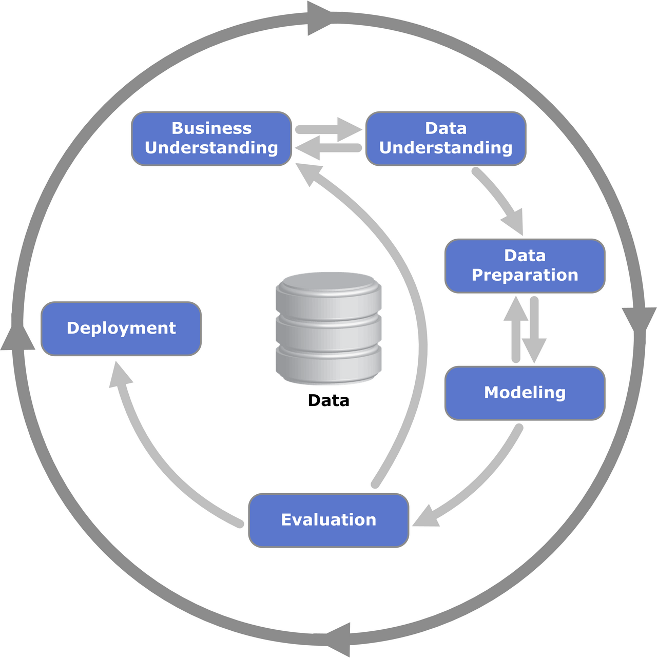
Figure 1. CRISP-DM Process Diagram. Source: Wikimedia Commons, “CRISP-DM Process Diagram”, public domain.
CRISP-DM is not a linear process, but an iterative one. In practice, phases continuously feed back into one another. During modeling, data quality issues may be discovered, forcing a return to the preparation phase. During evaluation, it may emerge that the business problem was incompletely specified, requiring a return to the first phase. Even after deployment, outcomes generate new strategic questions, restarting the cycle.
This iterative nature matches organizational realities: decision-making is a continuous process of refinement and learning. Thus, before creating tables, defining dimensions, or selecting tech stacks, teams must address questions such as:
- Which decisions does the organization wish to improve?
- Which metrics are critical?
- What time horizon needs to be analyzed?
The data architecture must be flexible and scalable, allowing new sources, metrics, and dimensions to be added as business needs evolve. Data architecture is not an end in itself; it is the technical foundation enabling operational data to become actionable knowledge within a continuous improvement loop.
CRISP-DM defines the analytical workflow, while the Data Warehouse provides a reliable organizational memory to support it. Not every CRISP-DM project requires a Data Warehouse, but when questions require combining multiple sources, comparing periods, and reusing consistent metrics, the data warehouse becomes a core element.
5.2 Data Warehouse
William H. Inmon (1996) defines a Data Warehouse as:
“A data warehouse is a subject-oriented, integrated, time-variant, and non-volatile collection of data in support of management’s decision-making process.”
The four properties in this definition are interconnected. Together, they explain why a Data Warehouse offers a coherent, long-lasting view of the business:
Subject-Oriented
Organizes data around business entities, such as customers, products, or students.
Integrated
Unifies codes, formats, business rules, and definitions across disparate systems.
Time-Variant
Preserves historical states to compare time frames and track long-term trends.
Non-Volatile
Prioritizes controlled loads and reads; history remains stable over time.
Conceptual Diagram: Inmon's classic properties convert fragmented operational data into a shared analytical memory.
A Data Warehouse is subject-oriented, meaning it is structured around core business entities rather than operational applications. For example, in an insurance company, the warehouse is organized around concepts like customer, policy, or claim, rather than separate software modules like auto insurance or life insurance. The focus is analyzing business entities rather than technical modules.
It is time-variant because it preserves historical data. Records are not overwritten as in transactional databases; new records are appended over time. This enables trend analysis across five, ten, or more years, answering questions regarding diagnosis trends or long-term sales growth patterns.
It is integrated because it consolidates data from multiple systems. If one system records gender as “M”/“F” and another as 0/1, they must be transformed into a unified format prior to storage. The same applies to differing date formats, currencies, or product codes. Integration involves data cleaning, transformation, and standardization.
Finally, it is non-volatile, meaning it is physically separate from operational systems. It primarily supports loading and querying operations, without frequent updates or operational transactions. Its purpose is analytical rather than operational.
Together, these properties ensure metrics retain consistent meaning across departments and time frames. For example, comparing student retention rates across cohorts is valid only if student identity, retention definitions, and academic calendars share unified rules, and historical records are preserved.
Reference:
Inmon, W. H. Building the Data Warehouse, 2nd ed., 1996.
6 Data Warehouse Architecture
A Data Warehouse is more than a set of query tables: it is an end-to-end data architecture designed to decouple daily operational activity from strategic analytics. This architecture integrates data across systems, maintains historical records, and provides structures optimized for decision support.
Decoupling protects both workloads: transactions run with low latency, while analytical queries can scan millions of rows without locking production databases. Between both worlds sits a transformation pipeline that tracks data provenance and transformation rules.
6.1 3-Tier Architecture
The classic Data Warehouse architecture is represented as a three-tier logical model. These tiers correspond to functional layers within the data ecosystem rather than separate physical servers.
LAYER 1
Operational Sources
ERP · CRM · APIs · CSV · Logs
Priority: Accurately record every event.
LAYER 2
Integration
Extract → Validate → Standardize → Load
Priority: Quality, traceability, and shared rules.
LAYER 3
Analytical Consumption
Data Marts · Models · BI · Analytics
Priority: Answer questions quickly and consistently.
Architectural Diagram: Each tier addresses a specific gap: data access, data consistency, and business utility.
Operational Layer.
This level houses systems supporting daily organization activities. In an enterprise, these include ERP systems logging sales and billing, CRMs managing customers, academic portals storing grades, or hospital EHR systems documenting medical visits. Flat files (CSV, Excel), external public APIs, and application log streams also sit in this layer.The goal here is transactional: recording events quickly, consistently, and securely. It is not designed for deep historical analysis or complex aggregations. A hospital system can track today’s patient visits, but is not optimized to analyze a decade of diagnostic trends.
Integration Layer (ETL / Data Integration Layer).
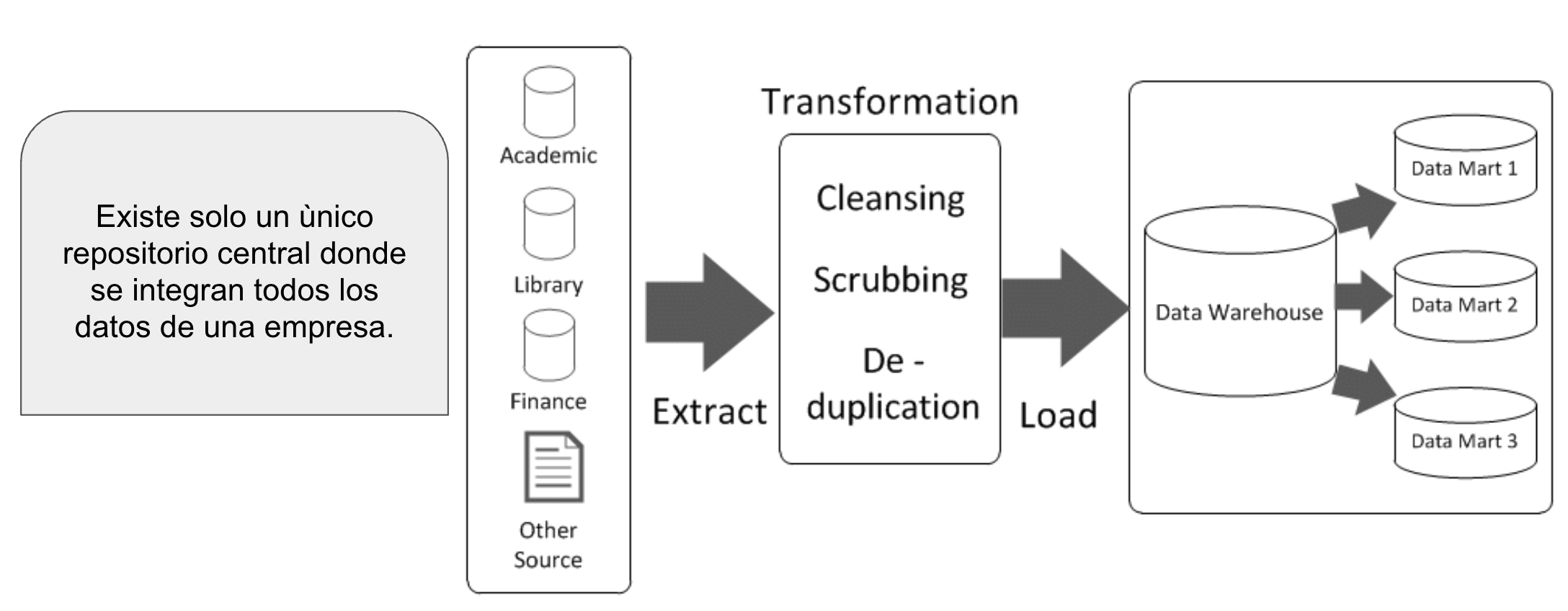
This layer forms the technical core of the Data Warehouse, executing extraction, cleaning, transformation, and loading processes. Inconsistencies are resolved here: gender codes (“M/F” vs 0/1) are normalized, date formats standardized, and currencies converted.Additionally, duplicates are removed, surrogate keys generated, and business rules applied to consolidate data. Depending on architectural choices, this layer can manifest as a centralized Enterprise Data Warehouse (EDW) where data is unified before presentation, or as pipelines feeding domain-specific dimensional models directly. In both cases, its role is guaranteeing enterprise-wide consistency and quality.
Presentation / Analytics Layer.
Data in this tier has been integrated and structured for analysis. Data marts, dimensional models (star schemas), BI dashboards, and visualization tools operate here. Analysts, executives, and business leads interact with this layer to answer strategic questions.For example, a healthcare network can analyze annual patient volumes by clinic, wait times by specialty, or regional diagnostic distributions. Crucially, data is optimized for querying, aggregation, and time-series comparisons rather than transaction processing.
6.2 Data Mart
A Data Mart is a specialized subset of a Data Warehouse focused on a specific business domain. While a Data Warehouse integrates enterprise-wide data, a Data Mart focuses on a domain like sales, finance, human resources, or academic tracking.
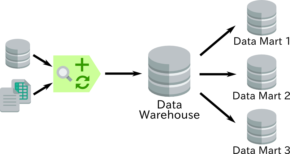
For instance, a university might deploy an academic Data Mart containing enrollment, grade, and credit fact tables linked to student, course, and time dimensions. A commercial enterprise might build a sales Data Mart with transaction facts and product, customer, and regional dimensions.
The main purpose of a Data Mart is facilitating focused analysis and improving query performance for a business unit. They are commonly implemented using dimensional modeling (star schemas), which is optimized for reporting and aggregations.
Depending on the architectural strategy, Data Marts can be derived from a central Data Warehouse (top-down approach) or built iteratively per business process and linked via conformed dimensions (bottom-up approach).
A Data Mart is not merely a small warehouse. Its value depends on keeping metrics and dimensions consistent with the rest of the organization. A sales Data Mart and an inventory Data Mart can be analyzed together only if both define “product”, “store”, and “time” identically.
6.3 Data Warehouse vs. Data Lake
In modern data architecture, a Data Lake is often discussed alongside a Data Warehouse, though their roles differ.
A Data Lake is a centralized repository that stores data in its raw format—structured, semi-structured, or unstructured. Unlike a Data Warehouse, which requires cleaning and transformation before loading, a Data Lake follows a flexible approach: store data first, transform later when needed for analysis.
For example, a Data Warehouse holds cleaned, normalized sales tables ready for reporting. A Data Lake can store raw sensor telemetry, medical images, JSON logs, app event streams, or unparsed text.
The primary distinction lies in purpose:
- The Data Warehouse is built for structured analysis and business decision-making.
- The Data Lake is built for flexible, massive-scale storage, particularly supporting Big Data workloads and Data Science exploration.
In modern platforms, both often coexist: the Data Lake acts as a raw landing zone, while the Data Warehouse provides curated structures optimized for business intelligence.
Data Lake
Stores structured, semi-structured, and unstructured data, often in raw form.
Schema: Defined on read
Users: Data Engineers and Data Scientists
Strength: Flexibility and scale
Data Warehouse
Publishes integrated, historical, structured data with controlled business definitions.
Schema: Defined before consumption
Users: Analysts and Business Leads
Strength: Consistency and analytical performance
Modern Architecture: They complement each other; choosing only one is not mandatory.
Comparative Diagram: The main difference is not data volume, but data preparation level and consumption patterns.
7 Implementation Approaches: Kimball vs. Inmon
Two classic approaches exist for constructing an enterprise DW: Kimball and Inmon. Both appear as foundational references: Kimball for dimensional modeling and Inmon for Data Warehouse architecture.
Both approaches aim to deliver integrated, actionable information, but start from opposite directions. Kimball begins with specific business processes and connects them incrementally; Inmon begins with a central integrated core before publishing consumption models. The chosen path dictates where value emerges first and where architectural complexity resides.
Kimball · Bottom-up
Business Process→
Dimensional Data Mart→
Conformed Dimensions→
Enterprise DW
Inmon · Top-down
Enterprise Vision→
Integrated EDW→
Derived Data Marts→
Analytical Consumption
Comparative Diagram: Two paths to integration: delivering coordinated domains incrementally vs. consolidating an enterprise core first.
7.1 Kimball Approach (Bottom-up, Bus Architecture)
The Kimball approach prioritizes rapid value delivery via dimensional data marts (usually star schemas) built per business process. The core idea is integrating separate data marts through conformed dimensions—shared, standardized dimensions (for example, identical definitions of “Time” and “Product” across Sales and Returns).
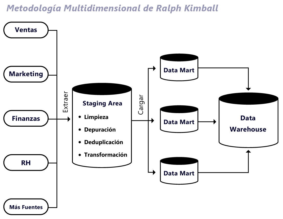
Key characteristics:
- Incremental implementation: Build one data mart (e.g., Sales) and expand iteratively (e.g., Inventory, Marketing).
- Target model: Dimensional, query-oriented.
- Focus on semantic layer: Consistent metric definitions (e.g., exact definition of “Net Sales”).
- High utility for BI/analytics from early stages.
Advantages:
- Fast delivery of tangible results to business users.
- Simple, high-performance query patterns.
- Natural alignment with business questions (the recommended starting point in this course).
Risks & Challenges:
- Requires strict discipline to enforce conformed dimensions; otherwise, isolated data silos emerge.
- Governance and integration can become complex if scaling without standards.
7.2 Inmon Approach (Top-down, EDW First)
The Inmon approach proposes constructing a centralized, integrated Enterprise Data Warehouse (EDW) first (typically using normalized models), then deriving domain data marts or dimensional views for analytical consumption.
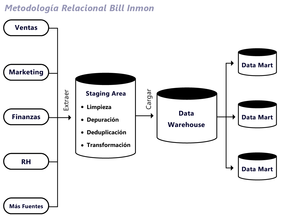
Key characteristics:
- Enterprise integration takes top priority: Unified corporate definitions from day one.
- Centralized repository harmonizing core entities and business rules (customer, product, organization).
- Data marts or dimensional models are downstream views derived from the EDW.
Advantages:
- High enterprise consistency and centralized metric control.
- Strong alignment with data governance, auditing, lineage, and compliance.
Risks & Challenges:
- Longer time-to-value as the EDW development cycle can be lengthy.
- Vulnerable to shifting business requirements because total integration is required before enabling use cases.
7.3 Selecting Between Kimball and Inmon
Choosing an approach should not be framed as “which is better”, but “which fits the organizational context, timeline, and data governance maturity”. Practical criteria:
- Analytics urgency and available resources
- If functional dashboards are needed quickly by a small or mid-sized team, Kimball is often more practical: build a first data mart and iterate.
- If an organization can sustain a large upfront investment and prioritizes unified corporate definitions from the start, Inmon may be preferable.
- Source data fragmentation and heterogeneity
- When dealing with disparate sources and conflicting definitions (e.g., “active customer” means different things across business units), an Inmon approach enforces central integration.
- If source systems are manageable and the goal is accelerating domain analytics (sales, academics, healthcare), Kimball performs well.
- Data governance, auditing, and lineage
- Strict regulatory or compliance auditing requirements favor the top-down, centralized framework.
- If data governance is maturing, an incremental approach is more realistic, provided conformed dimensions and metric glossaries are maintained.
- Nature of use cases
- Aggregated metrics and multidimensional navigation (trends, regional comparisons, cohorts) benefit from upfront dimensional modeling (Kimball).
- Enterprise master data management and complex cross-domain reconciliation favor Inmon or a strong core integration layer.
Modern data platforms frequently use a hybrid strategy: building an integrated core layer (EDW or core data layer) while exposing dimensional models for BI consumption. The critical goal is consistency: establishing a clear single source of truth for metrics and dimensions.
8 Practical Example: Faculty of Science
In a university setting, a grading system records transactional events such as student enrollments or final marks. However, analyzing a student’s full academic trajectory requires a broader perspective: integrating multiple semesters, cohorts, courses, curricula, and administrative data.
Academic operational systems handle daily processes—course registration, grade entry, transcript generation—but are ill-equipped for longitudinal or complex comparative analysis. For instance, answering:
- How has average student performance evolved across cohorts over the last ten years?
- Which student cohorts exhibit the highest attrition rates?
- Is there a correlation between admission channel and academic performance?
requires integrating data across systems while preserving historical context.
An Academic Data Warehouse consolidates this information into a historical, integrated repository optimized for strategic analysis.
8.1 Data Sources
In a Faculty of Science, relevant institutional data is typically spread across independent systems:
- Student Information Systems (SIS) recording enrollments, grades, and credits.
- Admissions Systems holding applicant data, admission scores, and educational background.
- Financial Systems managing tuition payments, scholarships, and financial aid.
- Human Resources Systems managing faculty records and teaching loads.
- External Files such as institutional surveys or academic evaluations.
Each system fulfills an operational need, but none offers a unified, longitudinal view of academic performance. Source fragmentation creates analytical barriers and metric inconsistencies.
8.2 Integration Processes (ETL)
Transforming operational data into strategic insight requires systematic integration.
Data is extracted periodically from source systems, cleaned, validated, standardized, and merged. For example, if a student’s name varies slightly across systems, the integration process identifies the individual and unifies their profile.
Institutional concepts—degree programs, course codes, academic terms, and department categories—are standardized across the repository.
The output is not a raw copy of operational databases, but a consolidated, clean dataset ready for historical analysis.
8.3 Data Warehouse Consolidation
Once integrated, data is stored in a central repository that preserves history and ensures consistency. This repository is not designed for transactional updates, but for analytical queries and longitudinal studies.
Architecturally, the academic Data Warehouse becomes the foundation for specialized analytical models—such as an academic data mart—from which institutional reports, dashboards, and research are generated.
Through consolidation, the Faculty can:
- Track student cohorts from admission to graduation.
- Measure failure and attrition rates by generation.
- Identify bottleneck courses with high fail rates.
- Evaluate performance trends over time.
- Combine academic KPIs with financial or administrative metrics.
The academic Data Warehouse transforms operational entries into strategic insight.
8.4 Academic DW Architectural Diagram
With this architecture, the Faculty can evaluate cohorts end-to-end, measure attrition rates, isolate high-failure courses, assess scholarship impacts on performance, and identify longitudinal trends. Unlike operational systems, the Data Warehouse unifies siloed data, preserves temporal history, supports multidimensional queries, and optimizes aggregations.
9 Conclusion
A Data Warehouse does not replace operational systems or record daily transactions. Its purpose is uniting fragmented data, preserving historical context, dismantling organizational silos, and powering complex analytics for strategic decision-making.
The next section explores multidimensional modeling, defining how analytical tables are structured and optimized for aggregated queries.
9.1 Visual Recapitulation: From Records to Analytics
To summarize, let us revisit the Faculty of Science case study and observe how an operational event gains analytical context through the architecture.
Sources
Student Records
Admissions
Human Resources
Surveys / CSV
➔
ETL Process
Extraction
Cleaning & Merging
Transformation
➔
Academic DW
Evaluation Facts
• Student Dimension
• Course Dimension
• Time Dimension
• Faculty Dimension
• Course Dimension
• Time Dimension
• Faculty Dimension
➔
Consumption
Academic Data Mart
Dashboards
Cohort Analysis
With this architecture, the Faculty can evaluate full student cohorts from entry to graduation, track attrition rates by generation, identify bottleneck courses, and analyze longitudinal performance trends.