49  Bayesian Classifiers

Supervised learning methods can be understood from two complementary perspectives. In a deterministic framework, the goal is learning a mapping \(f(\mathbf{x})\) that directly assigns instances to discrete classes or forecasts continuous responses. In a probabilistic framework, the primary focus is explicitly modeling uncertainty: rather than merely deciding a class label, we estimate the conditional probability of each candidate class given observed evidence. If no feature evidence is observed, optimal decision-making defaults to prior class probabilities.

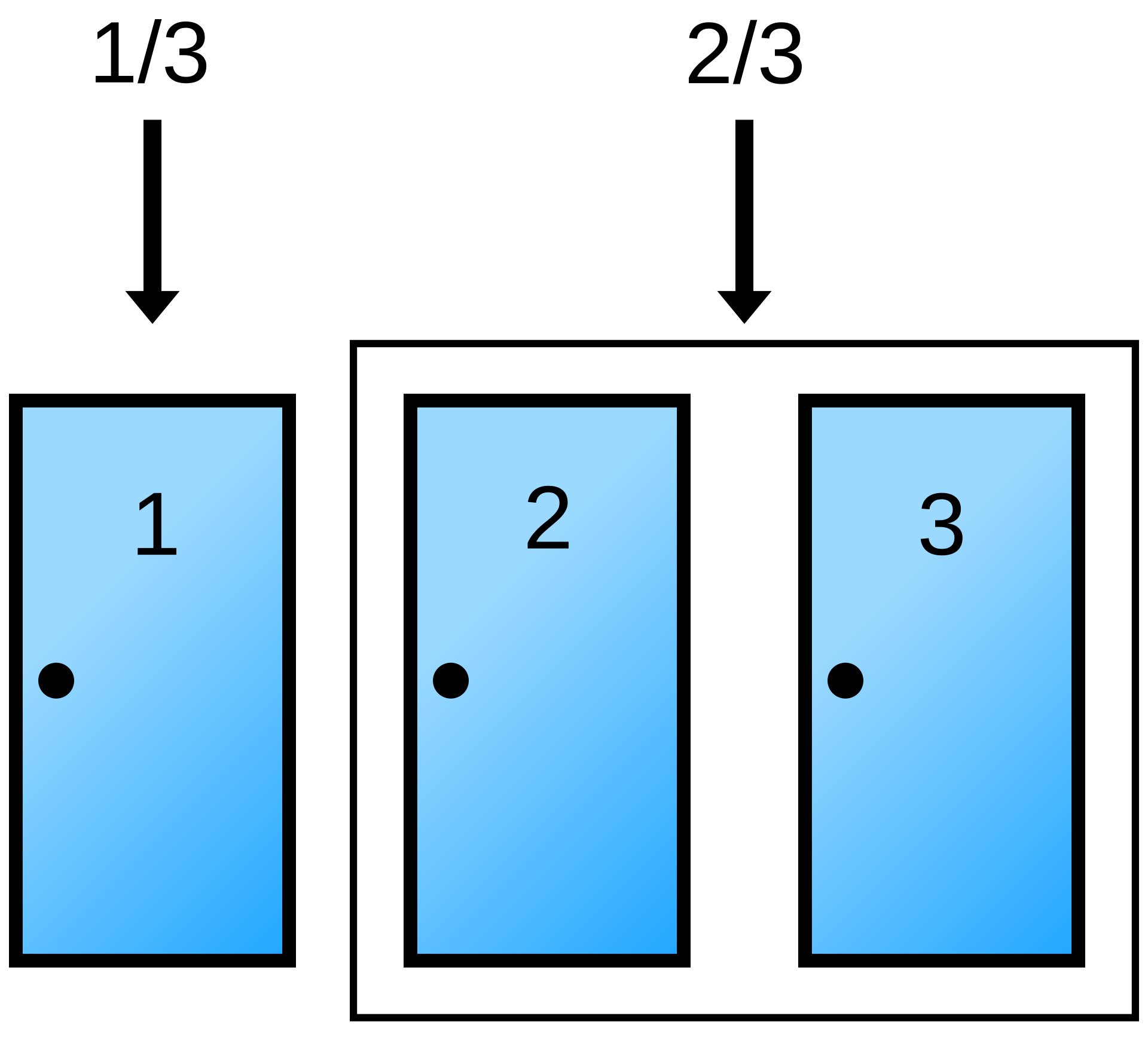
To illustrate, consider the classic Monty Hall game show scenario. A contestant is presented with 3 closed doors. Behind one door is a sports car; behind the other two are goats. Prior to receiving any hint, the prior probability of choosing the car is \(\frac{1}{3}\) across all three doors, making a uniform random choice optimal.

Prior probability of finding the car behind closed doors is \(\frac{1}{3}\), while finding a goat is \(\frac{2}{3}\).

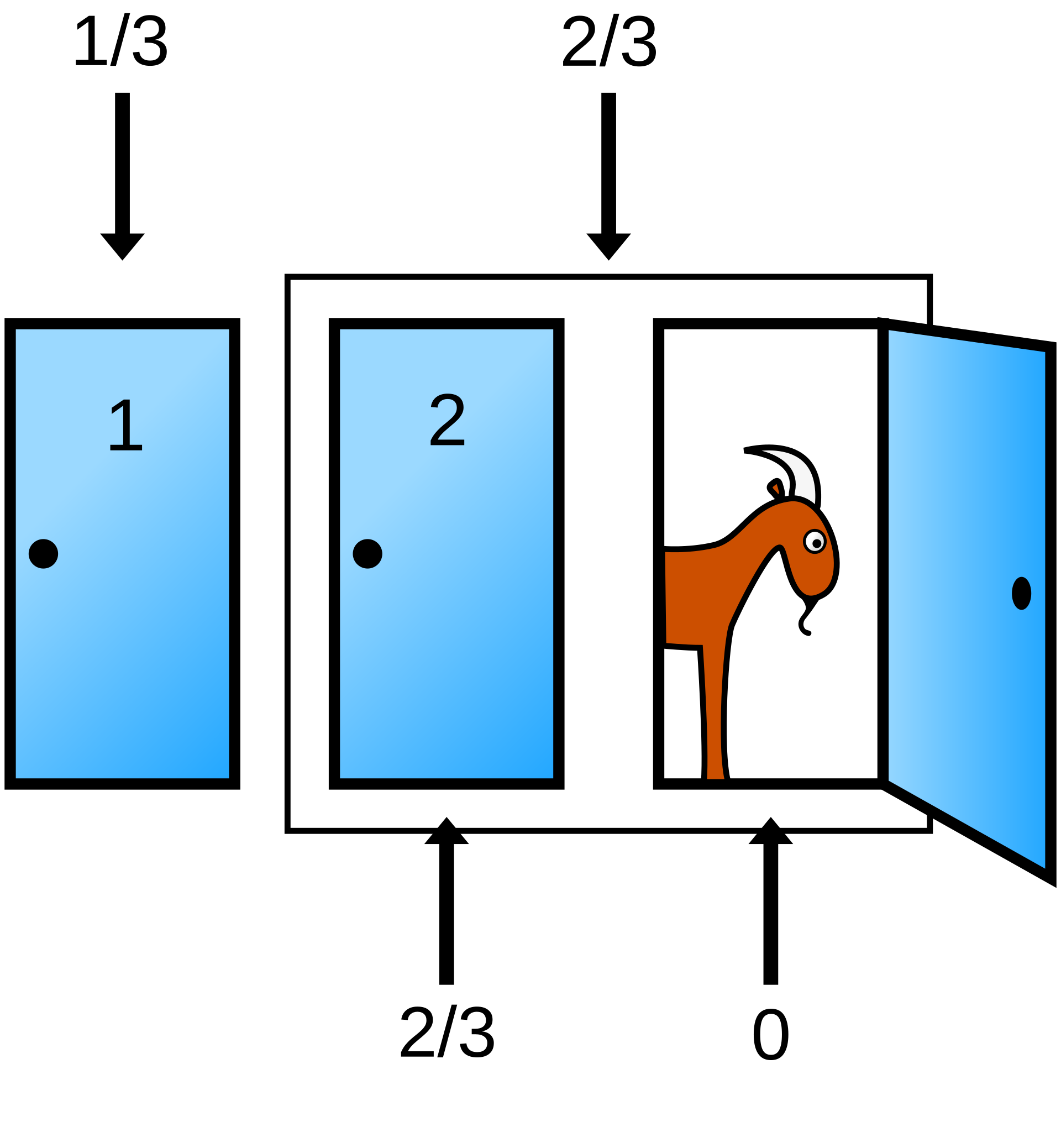
Suppose the contestant selects Door 1. The host (who knows what is behind each door) opens Door 3, revealing a goat. Should the contestant switch to Door 2? Intuition often incorrectly suggests a 50/50 chance between the two remaining closed doors.

Opening a goat door constraints the host to reveal a goat, shifting the conditional probability of winning by switching to \(\frac{2}{3}\).

Formally, prior probabilities before door opening are:

\[ P(A_1)=P(A_2)=P(A_3)=\frac{1}{3} \]

where \(A_i\) denotes the event that the car is behind Door \(i\).

The host knows the car’s location and always opens a door containing a goat. If the host has two goat doors to choose from (when the contestant initially picked the car), he chooses randomly between them.

Select your initial door:

The decision tree illustrates all possible game outcomes. High-probability branches (p = 1/3) contribute 2 units to state counts; low-probability branches (p = 1/6) contribute 1. Switching wins in 4 out of 6 weighted states.

When the host opens Door 3 revealing a goat, we condition on this evidence:

Case	Car Location	Prior \(P(A_i)\)	\(P(\text{Host opens Door 3} \mid A_i)\)	Joint Probability
1	Door 1	\(\frac{1}{3}\)	\(\frac{1}{2}\)	\(\frac{1}{6}\)
2	Door 2	\(\frac{1}{3}\)	\(1\)	\(\frac{1}{3}\)
3	Door 3	\(\frac{1}{3}\)	\(0\)	\(0\)

Total probability \(P(\text{Host opens Door 3}) = \frac{1}{6} + \frac{1}{3} + 0 = \frac{1}{2}\).

Applying Bayes’ Theorem:

\[ P(A_1 \mid \text{Host opens Door 3}) = \frac{1/6}{1/2} = \frac{1}{3} \]

\[ P(A_2 \mid \text{Host opens Door 3}) = \frac{1/3}{1/2} = \frac{2}{3} \]

Switching to Door 2 doubles the winning probability to \(\frac{2}{3}\). This highlights the core principle of Bayesian reasoning: updating initial beliefs upon observing new evidence.

import random
import plotly.graph_objects as go

def simular_monty_hall_plotly(n_simulaciones=10_000):
    puertas = [1, 2, 3]

    gana_quedandose = 0
    gana_cambiando = 0

    probabilidades_quedandose = []
    probabilidades_cambiando = []
    simulaciones = []

    for i in range(1, n_simulaciones + 1):
        puerta_auto = random.choice(puertas)
        eleccion_inicial = 1

        puertas_posibles_para_abrir = [
            puerta for puerta in puertas
            if puerta != eleccion_inicial and puerta != puerta_auto
        ]
        puerta_abierta = random.choice(puertas_posibles_para_abrir)

        puerta_cambio = [
            puerta for puerta in puertas
            if puerta != eleccion_inicial and puerta != puerta_abierta
        ][0]

        if eleccion_inicial == puerta_auto:
            gana_quedandose += 1
        if puerta_cambio == puerta_auto:
            gana_cambiando += 1

        probabilidades_quedandose.append(gana_quedandose / i)
        probabilidades_cambiando.append(gana_cambiando / i)
        simulaciones.append(i)

    fig = go.Figure()
    fig.add_trace(go.Scatter(
        x=simulaciones, y=probabilidades_quedandose,
        mode="lines", name="Stay Strategy",
        line=dict(color="#1f77b4", width=2)
    ))
    fig.add_trace(go.Scatter(
        x=simulaciones, y=probabilidades_cambiando,
        mode="lines", name="Switch Strategy",
        line=dict(color="#d62728", width=2)
    ))
    fig.add_hline(y=1/3, line_dash="dash", line_color="#1f77b4", annotation_text="Theoretical: 1/3")
    fig.add_hline(y=2/3, line_dash="dash", line_color="#d62728", annotation_text="Theoretical: 2/3")

    fig.update_layout(
        title="Monty Hall Simulation: Empirical Convergence to Bayesian Posteriors",
        xaxis_title="Number of Simulations",
        yaxis_title="Empirical Cumulative Win Rate",
        template="plotly_white",
        yaxis=dict(range=[0, 1])
    )
    fig.show()

simular_monty_hall_plotly(n_simulaciones=10_000)

1 Probabilistic Perspective on Classification

Given observation \(\mathbf{x}\in\mathbb{R}^d\) and candidate classes \(\Omega=\{\omega_1,\dots,\omega_c\}\), Bayes’ Theorem calculates posterior class probabilities \(P(\omega_i\mid \mathbf{x})\):

Definition. Posterior class probability \(P(\omega_i\mid \mathbf{x})\): \[ P(\omega_i\mid \mathbf{x}) = \frac{p(\mathbf{x}\mid \omega_i)P(\omega_i)}{p(\mathbf{x})} \tag{1}\]

where \(p(\mathbf{x}\mid\omega_i)\) is class-conditional likelihood, \(P(\omega_i)\) is prior class probability, and \(p(\mathbf{x}) = \sum_{j=1}^c p(\mathbf{x}\mid\omega_j)P(\omega_j)\) is marginal evidence.

Definition. Maximum A Posteriori (MAP) Decision Rule assigns instance \(\mathbf{x}\) to the class maximizing posterior probability: \[ \hat{\omega}(\mathbf{x}) = \arg\max_{\omega_i\in\Omega} P(\omega_i\mid\mathbf{x}) \tag{2}\]

import numpy as np

def clasificador_bayesiano(verosimilitudes, priors, clases):
    verosimilitudes = np.array(verosimilitudes, dtype=float)
    priors = np.array(priors, dtype=float)
    clases = np.array(clases)

    evidencia = np.sum(verosimilitudes * priors)
    posteriores = (verosimilitudes * priors) / evidencia

    indice_decision = np.argmax(posteriores)
    decision = clases[indice_decision]
    return posteriores, decision

clases = ["Normal", "Disease"]
verosimilitudes = [0.2, 0.4]
priors = [0.9, 0.1]

posteriores, decision = clasificador_bayesiano(verosimilitudes, priors, clases)
print(f"Posteriors: P(Normal|x) = {posteriores[0]:.3f}, P(Disease|x) = {posteriores[1]:.3f}")
print("MAP Decision:", decision)

Posteriors: P(Normal|x) = 0.818, P(Disease|x) = 0.182
MAP Decision: Normal

Bayesian Update — Prior → Posterior
Adjust prior P(ω₁) and likelihoods p(x|ω) to observe posterior shifts

P(ω₁) prior = 0.90

p(x|ω₁) = 0.20

p(x|ω₂) = 0.40

2 Minimum-Error Rate Classification

Under zero-one loss (where all classification errors incur unit cost), the MAP rule minimizes average error probability (Duda et al. 2001).

Definition. Conditional classification error \(P(e\mid\mathbf{x})\): \[ P(e\mid\mathbf{x})= \begin{cases} P(\omega_2\mid\mathbf{x}), & \text{if deciding }\omega_1,\\ P(\omega_1\mid\mathbf{x}), & \text{if deciding }\omega_2. \end{cases} \tag{3}\]

Likelihood ratio formulation:

\[ \ell(\mathbf{x})=\frac{p(\mathbf{x}\mid\omega_1)}{p(\mathbf{x}\mid\omega_2)} \gtrless_{\omega_2}^{\omega_1} \frac{P(\omega_2)}{P(\omega_1)}. \tag{4}\]

3 Naïve Bayes Classifier

Naïve Bayes simplifies multidimensional density estimation by assuming feature conditional independence given class \(\omega_i\) (McCallum and Nigam 1998; Murphy 2012):

Definition. Naïve Bayes Conditional Independence Assumption: \[ p(\mathbf{x}\mid\omega_i)=p(x_1,x_2,\dots,x_d\mid\omega_i)=\prod_{k=1}^{d}p(x_k\mid\omega_i) \tag{5}\]

Log-likelihood MAP decision rule:

\[ \hat{\omega}(\mathbf{x})=\arg\max_i \left[\log P(\omega_i)+\sum_{k=1}^{d}\log p(x_k\mid\omega_i)\right]. \]

Multinomial Naïve Bayes for text incorporating Laplace smoothing parameter \(\alpha\):

\[ \theta_{ik} = \frac{N_{ik}+\alpha}{\sum_{r=1}^{d}N_{ir}+\alpha d}. \]

4 Gaussian Bayes Classifiers

Modeling class-conditional densities via multivariate normal distributions:

Definition. Multivariate Gaussian density \(\mathcal{N}(\boldsymbol{\mu}_i,\boldsymbol{\Sigma}_i)\): \[ p(\mathbf{x}\mid\omega_i) = \frac{1}{(2\pi)^{d/2}|\boldsymbol{\Sigma}_i|^{1/2}} \exp\left[-\frac{1}{2}(\mathbf{x}-\boldsymbol{\mu}_i)^T\boldsymbol{\Sigma}_i^{-1}(\mathbf{x}-\boldsymbol{\mu}_i)\right] \tag{6}\]

• Quadratic Discriminant Analysis (QDA): Distinct covariance matrices \(\boldsymbol{\Sigma}_i \neq \boldsymbol{\Sigma}_j\) yield quadratic decision boundaries.
• Linear Discriminant Analysis (LDA): Shared covariance matrix \(\boldsymbol{\Sigma}_i = \boldsymbol{\Sigma}\) yields linear decision hyperplanes (Fisher 1936; Hastie et al. 2009).

5 Bayesian Minimum-Risk Classification

When classification errors carry unequal costs, decision theory minimizes expected conditional risk (Berger 1985).

Definition. Loss Matrix \(\lambda_{ij} = \lambda(\alpha_i,\omega_j)\) and Conditional Risk \(R(\alpha_i\mid\mathbf{x})\): \[ R(\alpha_i\mid\mathbf{x})=\sum_{j=1}^{c}\lambda(\alpha_i,\omega_j)P(\omega_j\mid\mathbf{x}) \tag{7}\]

Minimum-risk decision rule selects action \(\alpha^*(\mathbf{x}) = \arg\min_i R(\alpha_i\mid\mathbf{x})\).

6 Minimax Criterion for Uncertain Priors

When prior probabilities \(P(\omega_i)\) are unknown or non-stationary, the Minimax criterion selects decision rules minimizing worst-case risk across all admissible prior distributions (Berger 1985):

\[ \alpha_{\text{minimax}} = \arg\min_{\alpha}\max_{\pi\in\Pi} R(\alpha;\pi). \tag{8}\]

7 Conclusions

Bayesian classification provides a rigorous framework for decision-making under uncertainty. The MAP rule minimizes misclassification rates under symmetric costs, while Minimum-Risk Bayes incorporates asymmetric domain loss functions. Naïve Bayes handles high-dimensional spaces efficiently, and Gaussian discriminant classifiers model continuous feature spaces.

8 References

Berger, James O. 1985. Statistical Decision Theory and Bayesian Analysis. 2nd ed. Springer.

Duda, Richard O., Peter E. Hart, and David G. Stork. 2001. Pattern Classification. 2nd ed. Wiley.

Fisher, Ronald A. 1936. “The Use of Multiple Measurements in Taxonomic Problems.” Annals of Eugenics 7 (2): 179–88. https://doi.org/10.1111/j.1469-1809.1936.tb02137.x.

Hastie, Trevor, Robert Tibshirani, and Jerome Friedman. 2009. The Elements of Statistical Learning: Data Mining, Inference, and Prediction. 2nd ed. Springer Series in Statistics. Springer. https://doi.org/10.1007/978-0-387-84858-7.

McCallum, Andrew, and Kamal Nigam. 1998. “A Comparison of Event Models for Naive Bayes Text Classification.” AAAI-98 Workshop on Learning for Text Categorization, 41–48.

Murphy, Kevin P. 2012. Machine Learning: A Probabilistic Perspective. MIT Press.