28 Multivariate Exploratory Data Analysis: Theory and Visualization
Exploratory data analysis (EDA) has evolved significantly in recent years. While classic approaches focused on descriptive statistics and basic visualizations, modern multivariate EDA recognizes that real-world data is inherently high-dimensional and that understanding it requires integrating multiple analytical levels in a structured manner.
29 The Curse of Dimensionality
When the number of variables \(p\) grows, spatial geometry becomes deeply counterintuitive. The phenomenon known as the curse of dimensionality (Bellman, 1957) describes how spatial volume expands so rapidly that data points inevitably become sparse.
Consider a hypersphere of radius \(r\) inscribed within a hypercube of side length \(2r\) in \(\mathbb{R}^d\). The ratio of sphere volume to hypercube volume is:
\[ \frac{V_{\text{sphere}}}{V_{\text{cube}}} = \frac{\pi^{d/2} r^d}{\Gamma(d/2 + 1) \cdot (2r)^d} = \frac{\pi^{d/2}}{2^d \, \Gamma(d/2 + 1)} \]
In 2 and 3 dimensions, this ratio is relatively large (~78% and ~52% respectively), as shown in the following interactive visualization where \(r=1\).
However, this ratio tends to zero as \(d \to \infty\). This means that most of the hypercube’s volume concentrates in the corners, while the sphere (representing the region of interest) occupies a diminishing fraction of the total space.
This implies that for high-dimensional data analysis, maintaining a fixed sampling density \(\rho\) in \(\mathbb{R}^d\) requires the number of observations to scale as:
\[ n \sim \rho \cdot L^d \]
With \(p = 20\) features, there are \(\binom{20}{2} = 190\) pairwise correlations. With \(p = 100\), there are 4,950. Manually inspecting every relationship becomes impossible. Thus, we need methods that compress information without sacrificing core structure.
30 Mathematical Foundations of PCA
Principal Component Analysis (PCA) is a dimensionality reduction technique that transforms a dataset with correlated features into a new system of uncorrelated variables called principal components. Each component is a linear combination of original features and represents a direction of maximum variance, preserving as much original data information as possible.
30.1 Mathematical Formulation and Procedure
Given a dataset \(X \in \mathbb{R}^{n \times p}\), where \(n\) is the number of samples and \(p\) the number of features, the process follows a precise sequence:
Standardization and Centering
To prevent measurement scales from distorting the analysis, variables are transformed to a shared scale:
- Centering: subtract the mean of each feature
- Scaling: divide by its standard deviation
This ensures each variable has zero mean and unit variance.
\[ \tilde{X}_{ij} = \frac{X_{ij} - \mu_j}{\sigma_j} \]
where:
- \(\mu_j\) is the mean of feature \(j\)
- \(\sigma_j\) is its standard deviation
- Centering: subtract the mean of each feature
Covariance Matrix Calculation: The sample covariance matrix \(S\) summarizes feature variability and pairwise relationships:
\[S = \frac{1}{n-1} \tilde{X}^T \tilde{X}\]
Element-wise:
\[s_{jk} = \frac{1}{n-1} \sum_{i=1}^n (x_{ij} - \mu_j)(x_{ik} - \mu_k)\]
where:
- \(s_{jj}\) represents the variance of feature \(j\)
- \(s_{jk}\) represents the covariance between features \(j\) and \(k\)
This matrix is symmetric and positive semi-definite, guaranteeing real, non-negative eigenvalues.
Spectral Decomposition: The eigenvalue problem is solved to identify principal directions: \[S \mathbf{v} = \lambda \mathbf{v}\] Here, \(\lambda\) represents the eigenvalues (explained variance in that direction) and \(\mathbf{v}\) the eigenvectors (loadings/directions).
Optimization and Ranking: The first principal component \(w_1\) is the eigenvector associated with the largest eigenvalue \(\lambda_1\). Subsequent components maximize remaining variance subject to orthogonality constraints: \(\lambda_1 \geq \lambda_2 \geq \cdots \geq \lambda_p\).
Projection and Reduction: Finally, original data points are projected onto the subspace spanned by the top \(k\) components: \[\mathbf{Z} = \tilde{X} \mathbf{V}_k\] where \(\mathbf{V}_k\) contains the first \(k\) ranked eigenvectors.
Each component captures a fraction of total data variance (\(\sum \lambda_j\)). The contribution of each component is measured by the Proportion of Variance Explained (PVE):
\[\text{PVE}_k = \frac{\lambda_k}{\sum_{j=1}^p \lambda_j}\]
This enables reducing dimensionality while retaining, for instance, 95% of cumulative original variance.
30.2 Practical Example: Step-by-Step Manual Calculation
We demonstrate the full process using a two-variable raw dataset (\(p=2\)):
Original Data Matrix: Suppose \(n=3\) observations across \(p=2\) features: \[X = \begin{pmatrix} 2 & 3 \\ 3 & 4 \\ 4 & 5 \end{pmatrix}\]
Data Centering: Column means are \(\bar{x}_1 = 3\) and \(\bar{x}_2 = 4\). Subtracting means yields \(\tilde{X}\): \[\tilde{X} = \begin{pmatrix} 2-3 & 3-4 \\ 3-3 & 4-4 \\ 4-3 & 5-4 \end{pmatrix} = \begin{pmatrix} -1 & -1 \\ 0 & 0 \\ 1 & 1 \end{pmatrix}\]
Covariance Matrix (\(S\)): Applying \(S = \frac{1}{n-1} \tilde{X}^T \tilde{X}\) with \(n-1 = 2\): \[S = \frac{1}{2} \begin{pmatrix} -1 & 0 & 1 \\ -1 & 0 & 1 \end{pmatrix} \begin{pmatrix} -1 & -1 \\ 0 & 0 \\ 1 & 1 \end{pmatrix} = \frac{1}{2} \begin{pmatrix} 2 & 2 \\ 2 & 2 \end{pmatrix} = \begin{pmatrix} 1 & 1 \\ 1 & 1 \end{pmatrix}\]
Eigenvalue Computation (\(\lambda\)): Solving \(\det(S - \lambda I) = 0\): \[\det \begin{pmatrix} 1-\lambda & 1 \\ 1 & 1-\lambda \end{pmatrix} = (1-\lambda)^2 - 1 = 0 \implies \lambda^2 - 2\lambda = 0\] Yielding \(\lambda_1 = 2\) and \(\lambda_2 = 0\). Total variance is \(2+0=2\). The first component explains 100% of variance.
Eigenvector Computation (\(\mathbf{v}\)): For \(\lambda_1 = 2\), solving \((S - 2I)\mathbf{v}_1 = 0\): \[\begin{pmatrix} -1 & 1 \\ 1 & -1 \end{pmatrix} \begin{pmatrix} v_{11} \\ v_{21} \end{pmatrix} = 0 \implies v_{11} = v_{21}\] Normalizing so \(\|v\|=1\): \(v_1 = \begin{pmatrix} 1/\sqrt{2} \\ 1/\sqrt{2} \end{pmatrix} \approx \begin{pmatrix} 0.707 \\ 0.707 \end{pmatrix}\).
Data Projection (\(k=1\)): Projecting centered data onto PC1: \(Z = \tilde{X} v_1\): \[Z = \begin{pmatrix} -1 & -1 \\ 0 & 0 \\ 1 & 1 \end{pmatrix} \begin{pmatrix} 0.707 \\ 0.707 \end{pmatrix} = \begin{pmatrix} -1.414 \\ 0 \\ 1.414 \end{pmatrix}\]
Conclusion: Since original data points were perfectly colinear (\(x_2 = x_1 + 1\)), PCA reduces dimensionality from 2D to 1D with zero information loss.
30.3 Step-by-Step Interactive Visualizations
- Original Data Matrix
\[ X = \begin{pmatrix} 2 & 3 \\ 3 & 4 \\ 4 & 5 \end{pmatrix} \]
Code
import numpy as np
import plotly.graph_objects as go

X = np.array([[2,3],[3,4],[4,5]])

fig = go.Figure()
fig.add_trace(go.Scatter(
    x=X[:,0], y=X[:,1],
    mode='markers+text',
    text=['P1','P2','P3'],
    textposition='top center'
))
fig.update_layout(title="Original Data")
fig.show()- Data Centering
\[ \tilde{X} = \begin{pmatrix} -1 & -1 \\ 0 & 0 \\ 1 & 1 \end{pmatrix} \]
Code
X_centered = X - X.mean(axis=0)

fig = go.Figure()
fig.add_hline(y=0)
fig.add_vline(x=0)

fig.add_trace(go.Scatter(
    x=X_centered[:,0], y=X_centered[:,1],
    mode='markers+text',
    text=['P1','P2','P3'],
    textposition='top center'
))

fig.update_layout(title="Centered Data")
fig.show()- Covariance Matrix Calculation
\[ S = \begin{pmatrix} 1 & 1 \\ 1 & 1 \end{pmatrix} \]
Code
S = np.cov(X_centered, rowvar=False)

fig = go.Figure(data=go.Heatmap(
    z=S,
    text=S.round(2),
))

fig.update_layout(title="Covariance Matrix")
fig.show()- Eigenvalues
\[ \lambda_1 = 2, \quad \lambda_2 = 0 \]
Code
eigvals, eigvecs = np.linalg.eig(S)

fig = go.Figure()
fig.add_trace(go.Bar(
    x=['λ1','λ2'],
    y=eigvals
))

fig.update_layout(title="Variance per Component")
fig.show()- Eigenvectors
\[ v_1 \approx \begin{pmatrix} 0.707 \\ 0.707 \end{pmatrix} \]
Code
v1 = eigvecs[:, np.argmax(eigvals)]
t = np.linspace(-2,2,100)

fig = go.Figure()

fig.add_trace(go.Scatter(
    x=X_centered[:,0], y=X_centered[:,1],
    mode='markers'
))

fig.add_trace(go.Scatter(
    x=t*v1[0],
    y=t*v1[1],
    mode='lines',
    name='PC1'
))

fig.update_layout(title="Principal Direction (PC1)")
fig.show()- Data Projection
\[ Z = \begin{pmatrix} -1.414 \\ 0 \\ 1.414 \end{pmatrix} \]
Code
Z = X_centered @ v1

fig = go.Figure()

fig.add_trace(go.Scatter(
    x=Z,
    y=[0,0,0],
    mode='markers+text',
    text=['P1','P2','P3'],
    textposition='top center'
))

fig.update_layout(title="Projected Data on PC1")
fig.show()- Conclusion
- All variance concentrates along a single axis
- PCA compresses 2D to 1D seamlessly
- PC1 aligns with the line connecting the data points; PC2 contains zero variance.
31 PCA and Singular Value Decomposition (SVD)
Modern software libraries computing PCA (e.g., scikit-learn) do not perform direct eigendecomposition of \(S\). Instead, they apply Singular Value Decomposition (SVD) directly to the centered matrix \(\tilde{X}\), providing superior numerical stability and efficiency.
Any matrix \(\tilde{X} \in \mathbb{R}^{n \times p}\) can be decomposed as:
\[ \tilde{X} = U \Sigma V^T \]
where:
- \(U \in \mathbb{R}^{n \times n}\): orthogonal matrix of left singular vectors (columns = eigenvectors of \(\tilde{X}\tilde{X}^T\))
- \(\Sigma \in \mathbb{R}^{n \times p}\): diagonal matrix of singular values \(\sigma_1 \geq \sigma_2 \geq \cdots \geq \sigma_{\min(n,p)} \geq 0\)
- \(V \in \mathbb{R}^{p \times p}\): orthogonal matrix of right singular vectors (columns = eigenvectors of \(\tilde{X}^T\tilde{X}\))
The connection between SVD and PCA is direct:
\[ S = \frac{1}{n-1}\tilde{X}^T\tilde{X} = \frac{1}{n-1}(U\Sigma V^T)^T(U\Sigma V^T) = \frac{1}{n-1} V \Sigma^2 V^T \]
Therefore:
- Columns of \(V\) match the eigenvectors of \(S\) (principal component loadings)
- Eigenvalues of \(S\) equal \(\lambda_k = \sigma_k^2 / (n-1)\)
- Principal component scores are \(Z = \tilde{X}V = U\Sigma\)
Why use SVD over direct eigendecomposition?
- Numerical Precision: Forming \(\tilde{X}^T\tilde{X}\) squares the condition number \(\kappa\) to \(\kappa^2\), amplifying numerical errors.
- Efficiency when \(n \ll p\): Thin SVD operates directly on \(n \times p\) matrices without computing large \(p \times p\) covariance matrices.
- Algorithms: Golub-Reinsch SVD is more numerically stable than general non-symmetric eigendecomposition routines.
import numpy as np
from sklearn.preprocessing import StandardScaler
from sklearn.datasets import load_iris

X = load_iris().data
X_std = StandardScaler().fit_transform(X)

# Method 1: Eigendecomposition of S
S = np.cov(X_std.T)
eigenvalues, eigenvectors = np.linalg.eigh(S)
idx = np.argsort(eigenvalues)[::-1]
eigenvalues = eigenvalues[idx]
eigenvectors = eigenvectors[:, idx]

# Method 2: Direct SVD on X_std
U, sigma, Vt = np.linalg.svd(X_std, full_matrices=False)
lambda_svd = sigma**2 / (len(X_std) - 1)

print("Eigenvalues via S:  ", np.round(eigenvalues, 6))
print("Eigenvalues via SVD:", np.round(lambda_svd, 6))
print("Identical results:", np.allclose(eigenvalues, lambda_svd))
Eigenvalues via S: [2.938085 0.920165 0.147742 0.020854]
Eigenvalues via SVD: [2.938085 0.920165 0.147742 0.020854]
Identical results: True32 Practical Example: Iris Dataset Walkthrough
Dataset: Iris
We apply Scikit-learn to the classic Iris dataset, containing measurements of three iris species (setosa, versicolor, and virginica) across four numerical features:
- Sepal Length
- Sepal Width
- Petal Length
- Petal Width
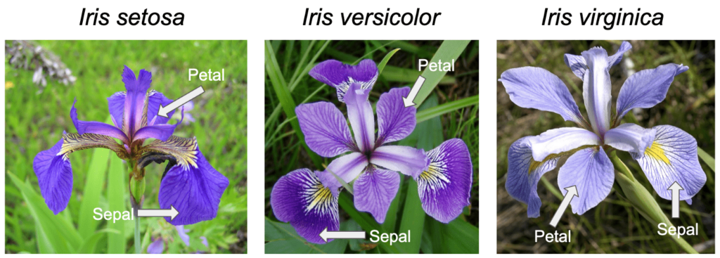
Code
iris = load_iris()
X = iris.data
y = iris.target
nombres = iris.target_names
feature_names = ['Sepal Length', 'Sepal Width', 'Petal Length', 'Petal Width']

df_iris = pd.DataFrame(X, columns=feature_names)
df_iris['Species'] = [nombres[i] for i in y]
df_iris.describe().round(3)| Sepal Length | Sepal Width | Petal Length | Petal Width | |
|---|---|---|---|---|
| count | 150.000 | 150.000 | 150.000 | 150.000 |
| mean | 5.843 | 3.057 | 3.758 | 1.199 |
| std | 0.828 | 0.436 | 1.765 | 0.762 |
| min | 4.300 | 2.000 | 1.000 | 0.100 |
| 25% | 5.100 | 2.800 | 1.600 | 0.300 |
| 50% | 5.800 | 3.000 | 4.350 | 1.300 |
| 75% | 6.400 | 3.300 | 5.100 | 1.800 |
| max | 7.900 | 4.400 | 6.900 | 2.500 |
Step 1: Standardization
Standardization is essential when features possess differing scales or units:
\[ z_{ij} = \frac{x_{ij} - \bar{x}_j}{s_j} \]
Post-standardization: \(\bar{z}_j = 0\) and \(s_{z_j} = 1\) for every feature \(j\).
Code
scaler = StandardScaler()
X_std = scaler.fit_transform(X)

df_check = pd.DataFrame({
    'Feature': feature_names,
    'Original Mean': X.mean(axis=0).round(3),
    'Original Std': X.std(axis=0).round(3),
    'Standardized Mean': X_std.mean(axis=0).round(10),
    'Standardized Std': X_std.std(axis=0).round(3)
})
df_check| Feature | Original Mean | Original Std | Standardized Mean | Standardized Std | |
|---|---|---|---|---|---|
| 0 | Sepal Length | 5.843 | 0.825 | -0.0 | 1.0 |
| 1 | Sepal Width | 3.057 | 0.434 | -0.0 | 1.0 |
| 2 | Petal Length | 3.758 | 1.759 | -0.0 | 1.0 |
| 3 | Petal Width | 1.199 | 0.760 | -0.0 | 1.0 |
Step 2: Covariance Matrix
Code
S = np.cov(X_std.T)

fig = go.Figure(data=go.Heatmap(
    z=S,
    x=feature_names,
    y=feature_names,
    colorscale='RdBu_r',
    zmid=0, zmin=-1, zmax=1,
    text=np.round(S, 3),
    texttemplate='%{text}',
    textfont=dict(size=13),
    hovertemplate='%{y} ↔ %{x}<br>cov = %{z:.3f}<extra></extra>',
    colorbar=dict(title='Covariance')
))
fig.update_layout(
    title="Covariance Matrix — Standardized Data (= Pearson Correlation Matrix)",
    height=420
)
fig.show()
Note
On standardized data, the covariance matrix is identical to the Pearson correlation matrix. Performing PCA on standardized data equals PCA on feature correlations.
Step 3: Eigendecomposition via SVD
Code
pca = PCA()
scores = pca.fit_transform(X_std)

eigenvalues = pca.explained_variance_
pve = pca.explained_variance_ratio_ * 100
pve_acum = np.cumsum(pve)

df_pca = pd.DataFrame({
    'Component': [f'PC{i+1}' for i in range(len(eigenvalues))],
    'Eigenvalue (λ)': eigenvalues.round(4),
    '% Variance': pve.round(2),
    '% Cumulative': pve_acum.round(2)
})
df_pca| Component | Eigenvalue (λ) | % Variance | % Cumulative | |
|---|---|---|---|---|
| 0 | PC1 | 2.9381 | 72.96 | 72.96 |
| 1 | PC2 | 0.9202 | 22.85 | 95.81 |
| 2 | PC3 | 0.1477 | 3.67 | 99.48 |
| 3 | PC4 | 0.0209 | 0.52 | 100.00 |
Step 4: Scree Plot
Code
fig = make_subplots(specs=[[{"secondary_y": True}]])

fig.add_trace(go.Bar(
    x=df_pca['Component'], y=df_pca['% Variance'],
    name='% Variance',
    text=[f"{v:.1f}%" for v in pve],
    textposition='outside'
), secondary_y=False)

fig.add_trace(go.Scatter(
    x=df_pca['Component'], y=pve_acum,
    mode='lines+markers',
    line=dict(width=2.5),
    marker=dict(size=9),
    name='% Cumulative'
), secondary_y=True)

fig.add_hline(y=80, line_dash="dash", line_color="gray",
              annotation_text="80%", secondary_y=True)

fig.update_yaxes(title_text="% Variance per Component", secondary_y=False)
fig.update_yaxes(title_text="% Cumulative Variance", range=[0, 110], secondary_y=True)
fig.update_layout(
    title="Scree Plot — Kaiser Rule: retain components with λ > 1",
    height=380
)
fig.show()
Tip
Criteria for selecting \(k\):
- Kaiser Rule: retain components with \(\lambda_k > 1\) (applies to standardized features)
- Cumulative Variance: retain components achieving at least 80% (or 90%) variance threshold
- Scree Plot Elbow: identify the bend where slope flattens
- Domain Interpretability: evaluate component domain meaning
Step 5: Biplot
A biplot overlays sample scores and feature loadings in the reduced PC space.
Code
loadings = pca.components_
scores_df = pd.DataFrame(scores[:, :2], columns=['PC1', 'PC2'])
scores_df['Species'] = [nombres[i] for i in y]

fig = go.Figure()

# Scores
for especie in nombres:
    mask = scores_df['Species'] == especie
    fig.add_trace(go.Scatter(
        x=scores_df.loc[mask, 'PC1'],
        y=scores_df.loc[mask, 'PC2'],
        mode='markers',
        marker=dict(size=7, opacity=0.7),
        name=especie
    ))

# Loadings vectors
escala = 3.0
for i, feat in enumerate(feature_names):
    fig.add_annotation(
        x=loadings[0, i] * escala,
        y=loadings[1, i] * escala,
        ax=0, ay=0,
        arrowhead=3, arrowwidth=2,
        xref='x', yref='y', axref='x', ayref='y',
        showarrow=True
    )
    fig.add_annotation(
        x=loadings[0, i] * escala * 1.15,
        y=loadings[1, i] * escala * 1.15,
        text=f"<b>{feat}</b>",
        showarrow=False,
        font=dict(size=11)
    )

fig.update_xaxes(title_text=f"PC1 ({pve[0]:.1f}%)",
                 zeroline=True, zerolinecolor='lightgray')
fig.update_yaxes(title_text=f"PC2 ({pve[1]:.1f}%)",
                 zeroline=True, zerolinecolor='lightgray',
                 scaleanchor='x')
fig.update_layout(
    title="Biplot: Scores + Loadings — Iris",
    height=480,
    legend=dict(title='Species')
)
fig.show()
Step 6: Detailed Loadings
Code
df_loadings = pd.DataFrame(
    loadings[:2].T,
    index=feature_names,
    columns=['PC1', 'PC2']
).round(4)

fig = make_subplots(
    rows=1, cols=2,
    subplot_titles=[
        "<b>Principal Component 1 (PC1)</b>",
        "<b>Principal Component 2 (PC2)</b>"
    ]
)

# PC1
fig.add_trace(go.Bar(
    x=feature_names,
    y=loadings[0],
    text=[f"{v:.3f}" for v in loadings[0]],
    textposition='outside'
), row=1, col=1)

# PC2
fig.add_trace(go.Bar(
    x=feature_names,
    y=loadings[1],
    text=[f"{v:.3f}" for v in loadings[1]],
    textposition='outside'
), row=1, col=2)

for c in [1, 2]:
    fig.update_yaxes(
        range=[-1.1, 1.1],
        zeroline=True,
        zerolinecolor='lightgray',
        row=1, col=c
    )
    fig.update_xaxes(
        tickangle=-25,
        row=1, col=c
    )

for ann in fig['layout']['annotations']:
    ann['font'] = dict(size=14)

fig.update_layout(
    showlegend=False,
    height=420,
    annotations=list(fig.layout.annotations) + [
        dict(
            x=0.5, y=-0.2,
            xref='paper', yref='paper',
            text="PC1 ≈ overall size | PC2 ≈ sepal structural contrast",
            showarrow=False,
            font=dict(size=12, color='gray'),
            xanchor='center'
        )
    ]
)

fig.show()
33 Advanced Example: Synthetic Noisy Trajectory
Imagine a particle traveling along a 3D helical trajectory measured by noisy sensors. We test whether PCA recovers the latent trajectory from multi-sensor data.
Step 1 — True Trajectory and Sensor Noise
Code
n_points = 500
t = np.linspace(-10, 10, n_points)

# Clean trajectory
x_clean = t
y_clean = np.cos(t)
z_clean = np.sin(t)

# Noisy measurements
sigma = 0.5
y_noise = y_clean + np.random.normal(0, sigma, n_points)
z_noise = z_clean + np.random.normal(0, sigma, n_points)

points = np.column_stack([x_clean, y_noise, z_noise])

fig = go.Figure()

fig.add_trace(go.Scatter3d(
    x=points[:, 0], y=points[:, 1], z=points[:, 2],
    mode='markers',
    marker=dict(size=3, color='steelblue', opacity=0.5),
    name='Noisy Measurements'
))

fig.add_trace(go.Scatter3d(
    x=x_clean, y=y_clean, z=z_clean,
    mode='lines',
    line=dict(color='crimson', width=4),
    name='True Trajectory'
))

fig.update_layout(
    title='Helical Trajectory: True Signal vs. Noisy Sensors',
    scene=dict(
        xaxis_title='X', yaxis_title='Y', zaxis_title='Z',
        yaxis=dict(range=[-5, 5]),
        xaxis=dict(range=[-11, 11])
    ),
    legend=dict(x=0.01, y=0.99),
    height=520
)
fig.show()
Step 2 — Multi-Sensor Projections
Code
def proyection(points, plane_point, plane_normal):
    n = plane_normal / np.linalg.norm(plane_normal)
    d = points - plane_point
    dist = d.dot(n)
    return points - np.outer(dist, n)

def plane_axes(plane_normal):
    n = plane_normal / np.linalg.norm(plane_normal)
    arb = np.array([1, 0, 0]) if abs(n[0]) < 0.9 else np.array([0, 1, 0])
    u = np.cross(n, arb)
    u /= np.linalg.norm(u)
    v = np.cross(n, u)
    v /= np.linalg.norm(v)
    return u, v

def sensor_reading(points, plane_point, plane_normal, noise_std=0.5):
    proj_3d = proyection(points, plane_point, plane_normal)
    u, v = plane_axes(plane_normal)
    proj_vectors = proj_3d - plane_point
    s = proj_vectors.dot(u) + np.random.normal(0, noise_std, len(points))
    t = proj_vectors.dot(v) + np.random.normal(0, noise_std, len(points))
    return s, t, proj_3d, u, v

def plane_mesh(plane_point, plane_normal, size=12, res=20):
    u, v = plane_axes(plane_normal)
    lin = np.linspace(-size, size, res)
    uu, vv = np.meshgrid(lin, lin)
    X = plane_point[0] + uu * u[0] + vv * v[0]
    Y = plane_point[1] + uu * u[1] + vv * v[1]
    Z = plane_point[2] + uu * u[2] + vv * v[2]
    return X, Y, Z

sensors = [
    dict(point=np.array([5., -6., 0.]),  normal=np.array([1., -1., 0.]),
         color='royalblue',  name='Sensor A'),
    dict(point=np.array([10., 0., 0.]),  normal=np.array([10., 0., 0.1]),
         color='seagreen',   name='Sensor B'),
    dict(point=np.array([3.,  3., 3.]),  normal=np.array([1.,  1., 1.]),
         color='darkorange', name='Sensor C'),
]

readings = []
for s in sensors:
    sc, tc, proj3d, u, v = sensor_reading(
        points, s['point'], s['normal'], noise_std=0.5
    )
    readings.append({'s': sc, 't': tc, 'proj3d': proj3d,
                     'u': u, 'v': v, **s})
Code
fig = go.Figure()

fig.add_trace(go.Scatter3d(
    x=x_clean, y=y_clean, z=z_clean,
    mode='lines', line=dict(color='crimson', width=4),
    name='True Trajectory'
))

fig.add_trace(go.Scatter3d(
    x=points[:, 0], y=points[:, 1], z=points[:, 2],
    mode='markers', marker=dict(size=2, color='lightgray', opacity=0.4),
    name='Original Measurements'
))

for r in readings:
    px_m, py_m, pz_m = plane_mesh(r['point'], r['normal'], size=10)
    fig.add_trace(go.Surface(
        x=px_m, y=py_m, z=pz_m,
        colorscale=[[0, r['color']], [1, r['color']]],
        opacity=0.15, showscale=False,
        name=f"Plane {r['name']}", showlegend=False
    ))
    fig.add_trace(go.Scatter3d(
        x=r['proj3d'][:, 0], y=r['proj3d'][:, 1], z=r['proj3d'][:, 2],
        mode='markers', marker=dict(size=2.5, color=r['color'], opacity=0.7),
        name=r['name']
    ))

fig.update_layout(
    title='Three Sensors Projecting Point Cloud Onto Respective Planes',
    scene=dict(xaxis_title='X', yaxis_title='Y', zaxis_title='Z',
               xaxis=dict(range=[-12, 12]),
               yaxis=dict(range=[-8, 8])),
    legend=dict(x=0.01, y=0.99),
    height=560
)
fig.show()
Step 3 — Multi-Sensor Feature Matrix
Code
data_matrix = np.column_stack([
    readings[0]['s'], readings[0]['t'],
    readings[1]['s'], readings[1]['t'],
    readings[2]['s'], readings[2]['t'],
])

col_labels = ['A_u', 'A_v', 'B_u', 'B_v', 'C_u', 'C_v']

corr = np.corrcoef(data_matrix.T)

fig = go.Figure(data=go.Heatmap(
    z=corr,
    x=col_labels, y=col_labels,
    colorscale='RdBu_r',
    zmid=0, zmin=-1, zmax=1,
    text=np.round(corr, 2),
    texttemplate='%{text}',
    textfont=dict(size=11),
    colorbar=dict(title='Correlation')
))

fig.update_layout(
    title='Correlation Across 6 Sensor Variables',
    height=420
)
fig.show()
Step 4 — PCA Decomposition
Code
pca_full = PCA(n_components=6)
components_full = pca_full.fit_transform(data_matrix)

explained = pca_full.explained_variance_ratio_
cumulative = np.cumsum(explained)

fig = make_subplots(specs=[[{"secondary_y": True}]])

fig.add_trace(go.Bar(
    x=[f'PC{i+1}' for i in range(6)],
    y=explained * 100,
    name='% Variance',
    text=[f'{v*100:.1f}%' for v in explained],
    textposition='outside',
    marker_color='steelblue'
), secondary_y=False)

fig.add_trace(go.Scatter(
    x=[f'PC{i+1}' for i in range(6)],
    y=cumulative * 100,
    mode='lines+markers',
    name='% Cumulative',
    line=dict(color='crimson', width=2.5),
    marker=dict(size=9)
), secondary_y=True)

fig.add_hline(y=90, line_dash='dash', line_color='gray',
              annotation_text='90%', secondary_y=True)

fig.update_yaxes(title_text="% Variance per Component", secondary_y=False)
fig.update_yaxes(title_text="% Cumulative Variance", range=[0, 110],
                 secondary_y=True)
fig.update_layout(
    title='Scree Plot: How Many Components Capture Signal?',
    height=400
)
fig.show()
Step 5 — 2D Projection
Code
pca_2d = PCA(n_components=2)
proj_2d = pca_2d.fit_transform(data_matrix)

fig = go.Figure()

fig.add_trace(go.Scatter(
    x=proj_2d[:, 0], y=proj_2d[:, 1],
    mode='markers',
    marker=dict(
        size=4, opacity=0.8,
        color=t,
        colorscale='Viridis',
        colorbar=dict(title='t (time)', len=0.6)
    ),
    name='Colored by t'
))

fig.update_xaxes(title_text='Principal Component 1',
                 zeroline=True, zerolinecolor='lightgray')
fig.update_yaxes(title_text='Principal Component 2',
                 zeroline=True, zerolinecolor='lightgray',
                 scaleanchor='x')
fig.update_layout(
    title=f'PC1 vs PC2 — {pca_2d.explained_variance_ratio_.sum()*100:.1f}% Total Variance',
    height=480
)
fig.show()
Step 6 — 3D Reconstruction
Code
pca_3d = PCA(n_components=3)
proj_3d = pca_3d.fit_transform(data_matrix)

fig = go.Figure()

fig.add_trace(go.Scatter3d(
    x=proj_3d[:, 0], y=proj_3d[:, 1], z=proj_3d[:, 2],
    mode='markers',
    marker=dict(
        size=3, opacity=0.7,
        color=t,
        colorscale='Viridis',
        colorbar=dict(title='t', len=0.5)
    ),
    name='Samples'
))

scale = proj_3d[:, 0].std() / x_clean.std()
fig.add_trace(go.Scatter3d(
    x=x_clean * scale,
    y=y_clean * proj_3d[:, 1].std(),
    z=z_clean * proj_3d[:, 2].std(),
    mode='lines',
    line=dict(color='crimson', width=4),
    name='True Trajectory (scaled)'
))

fig.update_layout(
    title=f'3D Projection — {pca_3d.explained_variance_ratio_.sum()*100:.1f}% Total Variance',
    scene=dict(
        xaxis_title='PC 1',
        yaxis_title='PC 2',
        zaxis_title='PC 3',
        xaxis=dict(range=[-15, 15]),
        yaxis=dict(range=[-7, 7]),
        zaxis=dict(range=[-7, 7])
    ),
    legend=dict(x=0.01, y=0.99),
    height=560
)
fig.show()
NoteCore Principle
PCA identifies directions of maximum variance. Because true signal variance dominates measurement noise (\(\text{SNR} \gg 1\)), top principal components capture signal while trailing components capture noise.
WarningKey Limitation
PCA assumes linear subspaces. Genuinely non-linear manifolds (e.g., Swiss Roll) require non-linear techniques such as UMAP or t-SNE.
34 Limitations of PCA
34.1 Linearity
PCA evaluates linear variance directions and cannot unroll non-linear manifolds.
Code
from sklearn.datasets import make_swiss_roll

X_swiss, t_swiss = make_swiss_roll(n_samples=800, noise=0.1, random_state=42)
X_swiss_std = StandardScaler().fit_transform(X_swiss)

pca_swiss = PCA(n_components=2)
scores_swiss = pca_swiss.fit_transform(X_swiss_std)

fig = make_subplots(1, 2,
    subplot_titles=['Swiss Roll (Original 3D)',
                    'PCA Projection (2D) — Structural Collapse'],
    specs=[[{'type': 'scatter3d'}, {'type': 'scatter'}]])

fig.add_trace(go.Scatter3d(
    x=X_swiss[:,0], y=X_swiss[:,1], z=X_swiss[:,2],
    mode='markers',
    marker=dict(size=3, color=t_swiss, colorscale='Viridis', opacity=0.7),
    showlegend=False
), row=1, col=1)

fig.add_trace(go.Scatter(
    x=scores_swiss[:,0], y=scores_swiss[:,1],
    mode='markers',
    marker=dict(size=4, color=t_swiss, colorscale='Viridis', opacity=0.7),
    showlegend=False
), row=1, col=2)

fig.update_layout(height=420)
fig.show()
34.2 Outlier Sensitivity
Minimizing mean squared reconstruction error renders PCA highly sensitive to outliers.
34.3 Class Unawareness
PCA is unsupervised and maximizes variance without considering class labels. Supervised alternatives like Linear Discriminant Analysis (LDA) explicitly maximize class separability.
Code
from sklearn.discriminant_analysis import LinearDiscriminantAnalysis

X_iris_std = StandardScaler().fit_transform(load_iris().data)
y_iris = load_iris().target
nombres_iris = load_iris().target_names

pca_comp = PCA(n_components=2)
scores_pca = pca_comp.fit_transform(X_iris_std)

lda = LinearDiscriminantAnalysis(n_components=2)
scores_lda = lda.fit_transform(X_iris_std, y_iris)

fig = make_subplots(1, 2,
    subplot_titles=['PCA (Unsupervised)', 'LDA (Supervised)'])

colors = px.colors.qualitative.Set1[:3]
for i, esp in enumerate(nombres_iris):
    mask = y_iris == i
    fig.add_trace(go.Scatter(
        x=scores_pca[mask, 0], y=scores_pca[mask, 1],
        mode='markers', marker=dict(color=colors[i], size=7, opacity=0.7),
        name=esp, legendgroup=esp
    ), row=1, col=1)
    fig.add_trace(go.Scatter(
        x=scores_lda[mask, 0], y=scores_lda[mask, 1],
        mode='markers', marker=dict(color=colors[i], size=7, opacity=0.7),
        name=esp, legendgroup=esp, showlegend=False
    ), row=1, col=2)

fig.update_layout(height=400,
    title="PCA vs LDA on Iris — LDA Optimizes Class Separation")
fig.show()
35 Beyond PCA: Non-Linear Techniques
Non-linear dimension reduction techniques like t-SNE and UMAP excel at preserving local manifold relationships.
We demonstrate on the MNIST handwritten digit dataset (784 dimensions).
Linear PCA fails to separate digit classes clearly on MNIST due to non-linear pixel dependencies.
35.1 t-SNE (t-Distributed Stochastic Neighbor Embedding)
t-SNE (van der Maaten & Hinton, 2008) minimizes Kullback-Leibler divergence between high-dimensional and low-dimensional pairwise probability distributions:
\[ \text{KL}(P \| Q) = \sum_{i \neq j} p_{ij} \log \frac{p_{ij}}{q_{ij}} \]
- Preserves local neighborhoods.
- Global inter-cluster distances are not meaningful.
- Key hyperparameter: perplexity (typically 5–50), controlling effective neighbor count:
\[ \text{Perplexity} = 2^{H(P_i)} \]
35.2 UMAP (Uniform Manifold Approximation and Projection)
UMAP (McInnes et al., 2018) relies on Riemannian geometry and category theory to preserve local and global manifold structures while offering faster computation.
| Feature | t-SNE | UMAP |
|---|---|---|
| Speed | Slow (\(O(n^2)\)) | Fast (\(O(n^{1.14})\)) |
| Global Structure | Poorly preserved | Better preserved |
| Out-of-sample mapping | No (transform() unavailable) |
Yes (transform() available) |
| Determinism | Non-deterministic | Deterministic with seed |
35.3 Method Selection Matrix
| Scenario | Recommended Method |
|---|---|
| Preprocessing before linear models | PCA |
| Exploratory visual inspection | t-SNE or UMAP |
| Large datasets (>50k samples) | UMAP |
| Transforming unseen test samples | PCA or UMAP |
| Linear component interpretability | PCA |
| Complex non-linear manifolds | UMAP |
| Supervised class discrimination | LDA |
36 Proposed Exercises
- PCA from Scratch: Implement PCA using only
numpy.linalg.svd. Verify eigenvalues and eigenvectors matchsklearn.decomposition.PCA. - Impact of Standardization: Apply PCA to Iris with and without feature scaling. Justify mathematically why loadings and variance ratios alter.
- Reconstruction Error: Given dataset \(X\) and rank-\(k\) PCA projection, reconstruct \(\hat{X} = Z_k W_k^T + \mu\). Plot Frobenius reconstruction error \(\|X - \hat{X}\|_F\) as a function of \(k\).
- t-SNE vs UMAP Benchmark: Compare t-SNE and UMAP on
sklearn.datasets.load_digitsregarding execution runtime and cluster separation quality. - Kaiser Rule Proof: Prove why Kaiser’s \(\lambda > 1\) rule strictly applies to standardized correlation matrices.